A Guide to Calculus They Hid from You in College
Mathematical analysis is, at its core, visual geometry — but universities disguise it as abstract algebra through epsilon-delta formalism. This guide reconstructs calculus the right way: through sequences, accumulation points, and geometric intuition.
"The essence of mathematics is not making simple things complicated, but making complicated things simple."
— S. Gudder
Have you ever wondered why objects in video games sometimes clip through textures? Or why financial models are so complex when trying to predict stock prices that seem sometimes smooth, sometimes jumpy? At the root of these seemingly different problems lies one and the same fundamental idea that the greatest minds of humanity struggled with for over two thousand years. The idea of continuity.
This is not just a fancy term from textbooks. This is a story about how we tried to connect the world of countable, separate objects with the world of smooth, indivisible motion. This is a story about a battle with infinity. I want to tell it the way it was never told to me in university: without quantifiers and deltas, through paradoxes and brilliant insights, and without the slightest loss of mathematical rigor. We will trace the path from Aristotle to the creators of calculus and see how one beautiful idea shaped our world.
Today you may also learn for the first time that the triumph of Cauchy's formalization of analysis over Heine's alternative is the single biggest reason why the concepts and ideas of mathematical analysis remain incomprehensible to the majority of students. Of the clear and intuitive language proposed by Heine — which requires absolutely no epsilons or deltas — only the Heine definition of limit survived in textbooks, and only because certain theorems simply cannot be proved without it. But what's even more interesting is that Cauchy's definition of limit is not needed for proofs at all!
After reading this article, you will be able to effortlessly and clearly understand roughly half of the first semester of a university course in mathematical analysis — possibly even more deeply than many calculus lecturers themselves.
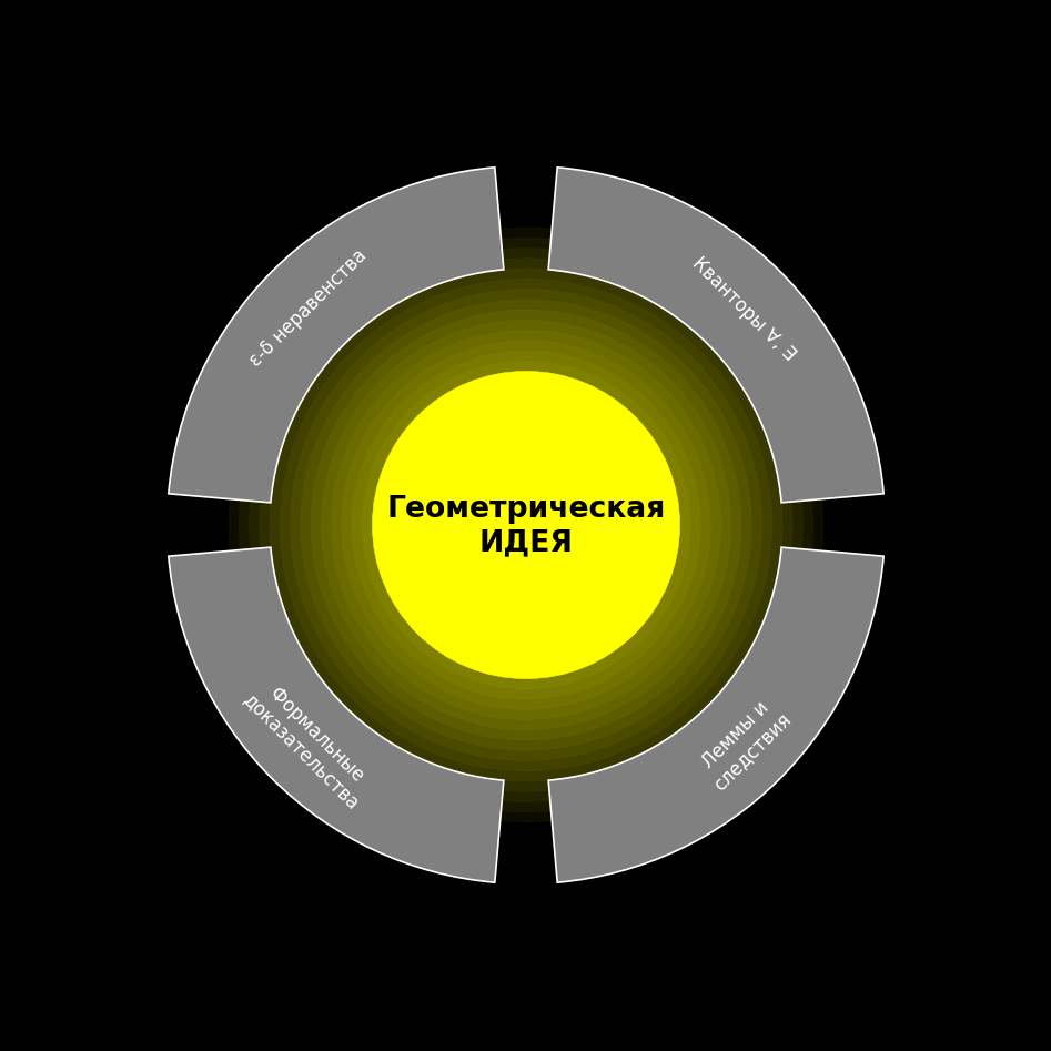
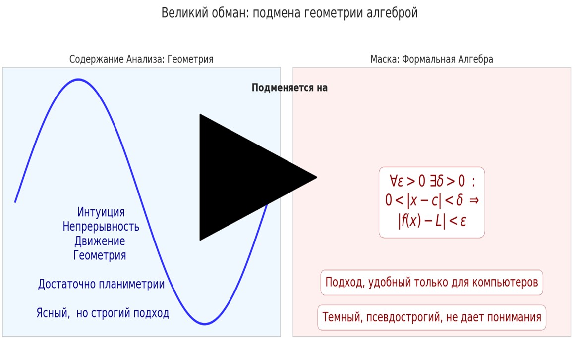
Prepare yourself for what may be the exposure of the greatest deception in modern higher education. Its essence is simple: by its very nature, mathematical analysis is visual geometry, but it is disguised as abstract algebra. As a result of this trick, a simple and clear subject becomes a dark forest even for many lecturers.
Preliminary Example
Let us prove that the limit of the function f(x) = 2x + 1 as x approaches 3 equals 7.
Proof #1: The Classical Cauchy Path (a wall of epsilon-delta)
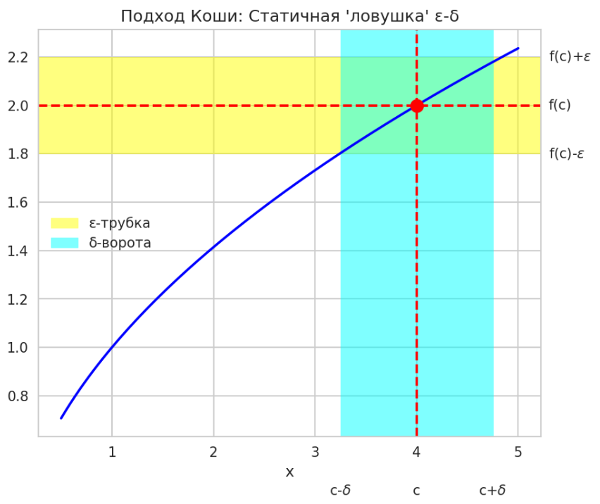
We need to prove that for any ε > 0 there exists δ > 0 such that if 0 < |x − 3| < δ, then |(2x + 1) − 7| < ε.
Consider |(2x + 1) − 7| = |2x − 6| = 2|x − 3|. We want 2|x − 3| < ε, which is equivalent to |x − 3| < ε/2.
So for any given ε > 0, we can choose δ = ε/2. Then if 0 < |x − 3| < δ, we get |x − 3| < ε/2, and consequently |(2x + 1) − 7| = 2|x − 3| < 2(ε/2) = ε.
Proved.
(Feel that? To prove an obvious thing, we had to "reverse-engineer" the inequality. It feels less like reasoning and more like fitting the answer.)
Proof #2: The Elegant Heine Path (logical reasoning)
- Take any sequence {xn} that converges to 3.
- By the definition of the limit of a sequence, this means {xn − 3} converges to 0.
- Consider the sequence of function values: {f(xn)} = {2xn + 1}.
- We need to prove that it converges to 7. To do this, look at the difference: {f(xn) − 7} = {(2xn + 1) − 7} = {2xn − 6} = {2(xn − 3)}.
- Since {xn − 3} converges to 0, the sequence {2(xn − 3)} converges to 0.
- And since {f(xn) − 7} converges to 0, the sequence {f(xn)} itself converges to 7.
(No tricks. Just straightforward reasoning, step by step, based on definitions. This is what genuine understanding looks like.)
Our Journey, Step by Step
The article is divided into three major parts:
- Part I: Origins of the Problem — from Aristotle to Cantor. The philosophical and mathematical history of the discrete-continuous divide.
- Part II: Taming Infinity. Foundational concepts: sets, numbers, continuity, cardinality.
- Part III: Building Proper Analysis — Without Epsilon-Delta. Constructing complete analysis using Heine's approach via sequence limits.
Why I Believe Calculus Is Taught Incorrectly
I moved to Yekaterinburg in 2020 during the COVID-19 pandemic and began teaching mathematical analysis there. The contrast with my previous experience at MFTI (Moscow Institute of Physics and Technology) was stark.
At MFTI, seminars functioned as genuine interactive learning sessions — problem-solving was tightly connected to theory, and students engaged with the material deeply. In Yekaterinburg, lectures bore no relation to seminars. Seminars consisted of rapidly working through Demidovich problems without explaining the underlying theory or theoretical connections.
Students couldn't even define basic concepts like "nested segments" or answer whether a segment contains itself. They panicked when given non-textbook homework problems because they couldn't copy solutions from standard answer guides. Students didn't want to know any of this theory!
I realized that the fundamental problem was not students' laziness but the curriculum itself. The reliance on Demidovich problem books meant all homework got copied from answer keys (the so-called "Antidemiovich"), preventing genuine learning. The texts were too difficult for weak students without the conceptual scaffolding.
Most critically, I identified that students struggle fundamentally with nested quantifiers (∀ε ∃δ...). This formalism serves as the obstacle to understanding analysis — for both students and even many calculus lecturers. The quantifier barrier is not essential to rigor; it is an artifact of choosing Cauchy's language over Heine's.
Part I. Origins of the Problem: From Aristotle to Cantor
Chapter 1. The Ancient Rift: Counting Stones versus a Flowing River
Humanity has always lived in two worlds simultaneously. In the first world, everything is separate and countable: five sheep, three soldiers, ten coins. These are objects that can be pointed to, labeled with numbers, and counted. This is the world of discrete quantities.
But there is a second world — the world of smooth and indivisible flow. A river flows, time passes, a line stretches. You can always insert another point between any two points. This is the world of continuous quantities.
For a long time, these two worlds seemed irreconcilable. Aristotle formulated the paradox that became the central problem for two millennia: can a continuous line be composed of indivisible points?

If points touch — they merge into one point, and the line collapses. If points don't touch — there are gaps between them, and continuity is destroyed. Both outcomes contradict the very idea of a continuum.
The ancient Greeks found a practical solution: they simply divided mathematics into two disciplines. Arithmetic dealt with the discrete (numbers), and geometry dealt with the continuous (figures). The two were never mixed. This avoided the paradox but never resolved it.
Centuries later, Newton and Leibniz created calculus through what amounted to "magical tricks" — methods that worked brilliantly in practice but lacked rigorous justification. For roughly 150 years, calculus operated on shaky foundations, producing correct results through procedures no one could fully explain.
Chapter 2. The Philosophical Key: Two Infinities and Hegel
To resolve the ancient paradox, we first need to understand infinity itself. It turns out there are two fundamentally different ways to conceive of it:
"Bad infinity" (a term from Spinoza): an unfinished process that never terminates. Counting 1, 2, 3, 4... and never stopping. This infinity is always incomplete, always reaching for something it can never grasp. It represents eternal incompleteness.
"True infinity": a self-sufficient, completed wholeness. Not the process of counting, but the complete concept of "all natural numbers" as a finished object. Not the endless extending of a line, but "the entire number line" as a single entity.
Georg Wilhelm Friedrich Hegel provided the philosophical framework that would prove decisive. His dialectical method — thesis, antithesis, synthesis — offered a way to reconcile seemingly irreconcilable opposites:
- Thesis (the Universal): The intuitive notion of a seamless, unbroken continuum — a whole without parts.
- Antithesis (the Particular): The attempt to construct a continuum from discrete points — parts without a whole. This crashes into Aristotle's paradox.
- Synthesis (the Specific): A new concept that is simultaneously a whole AND composed of elements — the unity of opposites.
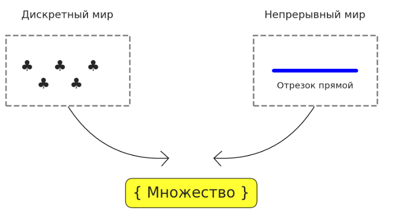
This philosophical framework was not merely abstract speculation. Mathematician Georg Cantor, reading Spinoza on the two types of infinity, recognized that a "set" perfectly embodies this Hegelian synthesis. A set is simultaneously a concrete, particular object AND contains infinite elements AS a completed totality.
Chapter 3. The Grand Unification: The Birth of the "Set"
Cantor's concept of "set" (Menge) unified the discrete and continuous under a single framework. This was the great breakthrough:
A set exhibits three aspects simultaneously:
- It is a particular, concrete object that we can refer to and work with.
- It consists of individual elements, addressing the requirement for discrete components.
- It embodies universal ideas (like "ALL points on a segment"), capturing "true infinity" as a completed whole.
The revolutionary consequence: sets became the universal mathematical language.
- A herd of sheep = a set
- A line segment = a set
Both are treated identically within formal theory, despite their intuitive differences. Everything became a set!
The ancient boundary between discrete and continuous was finally eliminated. Sets enabled rigorous comparison of infinities through bijection (one-to-one correspondence), which allowed mathematicians to distinguish countable infinities from uncountable ones — a distinction that would prove essential for understanding continuity.
Part II. Taming Infinity
Chapter 4. The Essence of Analysis: How to Catch Continuity by the Tail
Now we face the central question: how do we rigorously define continuity without relying on vague intuitions like "drawing a graph without lifting the pencil"? The challenge is subtle: on a continuous line, points have no "neighbors" — between any two points lie infinitely many others. So how do we detect a microscopic discontinuity?
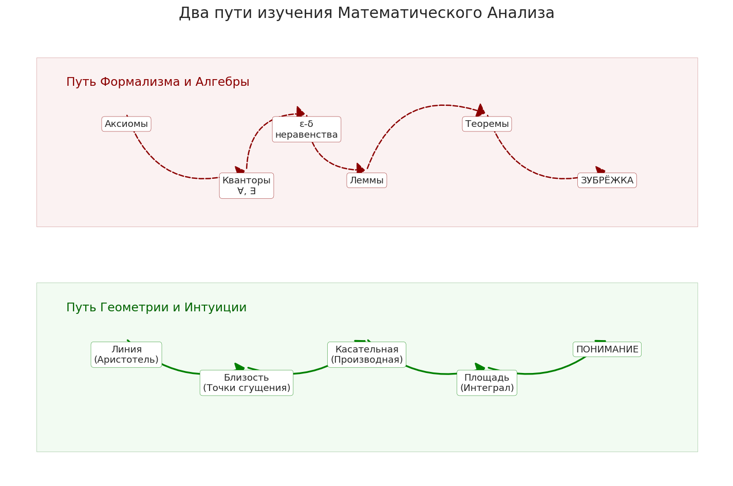
There are two competing approaches:
The Cauchy-Weierstrass approach: static epsilon-delta definitions that describe results rather than processes. For every ε > 0, there exists δ > 0 such that... This is powerful but opaque — it requires reverse-engineering inequalities rather than following natural logic.
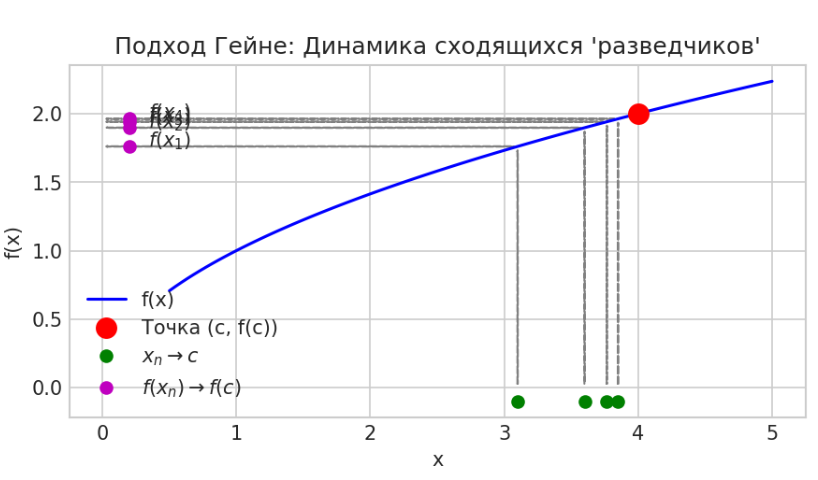
The Heine approach — a third path using the infinite process of approaching a point:
- Take ANY sequence {xn} converging to point c.
- Observe the function's response: a new sequence {f(xn)}.
- Verify: if f is continuous at c, then {f(xn)} → f(c).
Definition (Heine): A function f is continuous at point c if for any sequence {xn} converging to c, the sequence of values {f(xn)} converges to f(c).
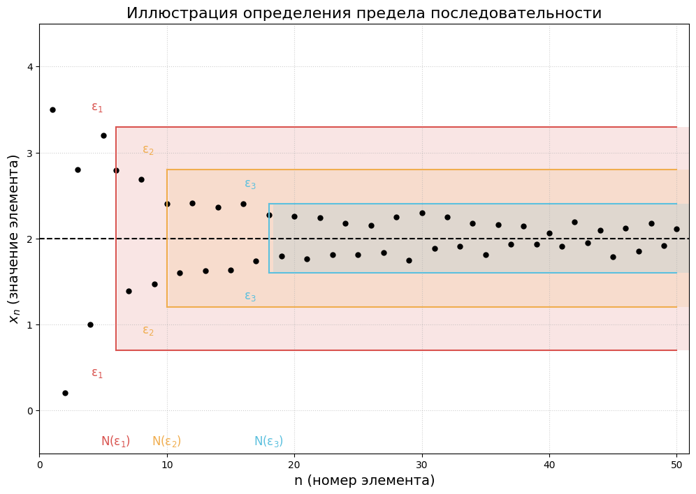
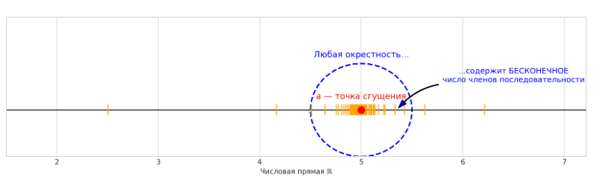
The conceptual innovation here is the "accumulation point" (or "condensation point"). Instead of a static picture, we use a dynamic concept: point a is a sequence's accumulation point when ANY arbitrarily small region around a contains infinitely many sequence elements.
Think of fireflies blinking in sequence. The accumulation point is where, no matter how much you zoom in, you always see infinitely many flashes.
The key distinction from Cauchy: Cauchy says "for every ε > 0 there exists δ > 0 such that..." (reverse-engineering inequalities). Heine says: the point approaches, the values approach, therefore continuous. It is natural, direct reasoning.
Chapter 5. Caution: Doors to the Foundations of Mathematics!
Cantor's naive definition of a set — "a collection of definite, distinct objects of our perception or thought, conceived as a unified whole" — sounds perfectly intuitive. But it conceals a logical abyss.
Russell's Paradox — The Catastrophe:
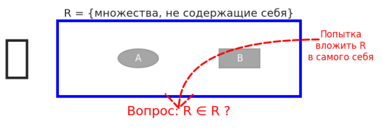
Consider R = "the set of all sets that do not contain themselves."
Does R contain itself?
- If YES: It violates the defining property (R should only contain sets that do NOT contain themselves).
- If NO: Then R satisfies its own defining criterion and must be in R.
Result: "A is true if and only if A is false" — logic itself collapses.
The Modern Solution — ZFC Axioms:
The Zermelo-Fraenkel set theory with the Axiom of Choice (ZFC) doesn't define "what a set is" but rather "how sets behave." It is a constitution for mathematics, not a semantic definition.
"A set is a fundamental object that is completely determined by the collection of its elements."
The key protective mechanism is the Axiom of Separation (Selection): you cannot simply declare "the universe of all objects with property X" into existence. Instead, you must take an already existing set A and extract a subset of elements satisfying property X. You can only "cut out" new subsets from legitimate, pre-existing sets.
This blocks Russell's paradox: creating the universal set R becomes an illegal operation. You cannot construct from a vacuum — only extract from what already exists.
Chapter 6. Defining Numbers: Building a World from Nothing
Here is a paradox: all of mathematics rests on set theory, which begins with nothing more than the empty set ∅ and operations on sets. So where do numbers come from? We cannot simply assert "numbers exist" — we must construct them using only the tools available.
Von Neumann's Construction — A Stroke of Genius:
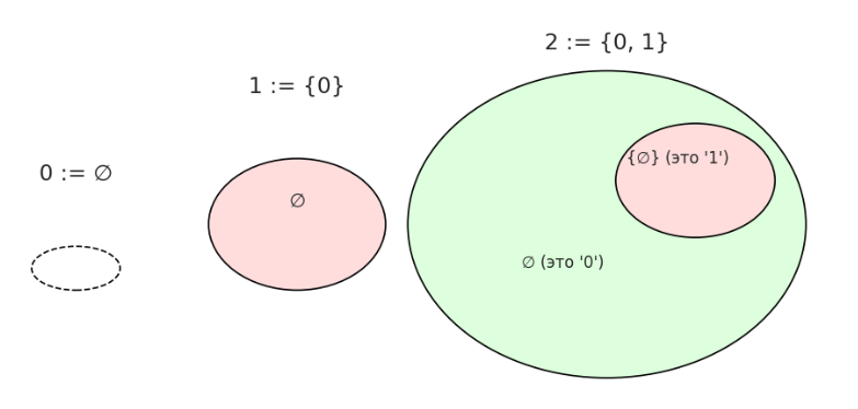
Each natural number is identified with the set of all preceding numbers:
- 0 := ∅ (the empty set = zero)
- 1 := {0} = {∅} (one element: zero itself)
- 2 := {0, 1} = {∅, {∅}} (two elements: zero and one)
- 3 := {0, 1, 2} (three elements)
The pattern: each natural number n equals the set of all numbers less than n.
This construction proves that arithmetic can be founded entirely on set theory. From here, further constructions build the rest:
- Integers ℤ: pairs (a, b) representing a − b
- Rationals ℚ: pairs (m, n) representing m/n, with equivalence relations
- Reals ℝ: require a new axiom — the axiom of completeness
The significance is profound: everything — all of mathematics — can be rigorously built from nothing (the empty set) using pure logic and set operations. No intuitive assumptions are needed. The foundation becomes unassailable.
Chapter 7. Number Sets: Plugging the Holes in Reality
The ancient Greeks believed all quantities could be reduced to ratios of integers. But the Pythagorean theorem revealed that √2 cannot be expressed as a fraction p/q. This irrational number represents an actual length — the diagonal of a unit square — yet has no rational representation.
The rational number line, despite being infinitely dense (between any two fractions lie infinitely many others), is riddled with "holes" where irrationals should be. The continuous line is actually a sieve.
Dedekind's Solution — The Completeness Axiom:
Richard Dedekind formulated the axiom that transforms the number line from a sieve into a true continuum:
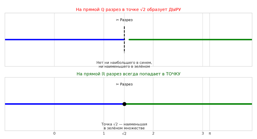
"Any cut of the number line passes through some point; there are no gaps."
Dedekind's Cut illustrated:
- On ℚ: A cut at √2 creates set A (all rationals less than √2) and set B (all rationals greater). Neither set has a boundary element — the knife passes through empty space.
- On ℝ: Any cut intersects exactly at some real number. The completeness axiom guarantees this — there are no gaps.
This axiom has equivalent formulations:
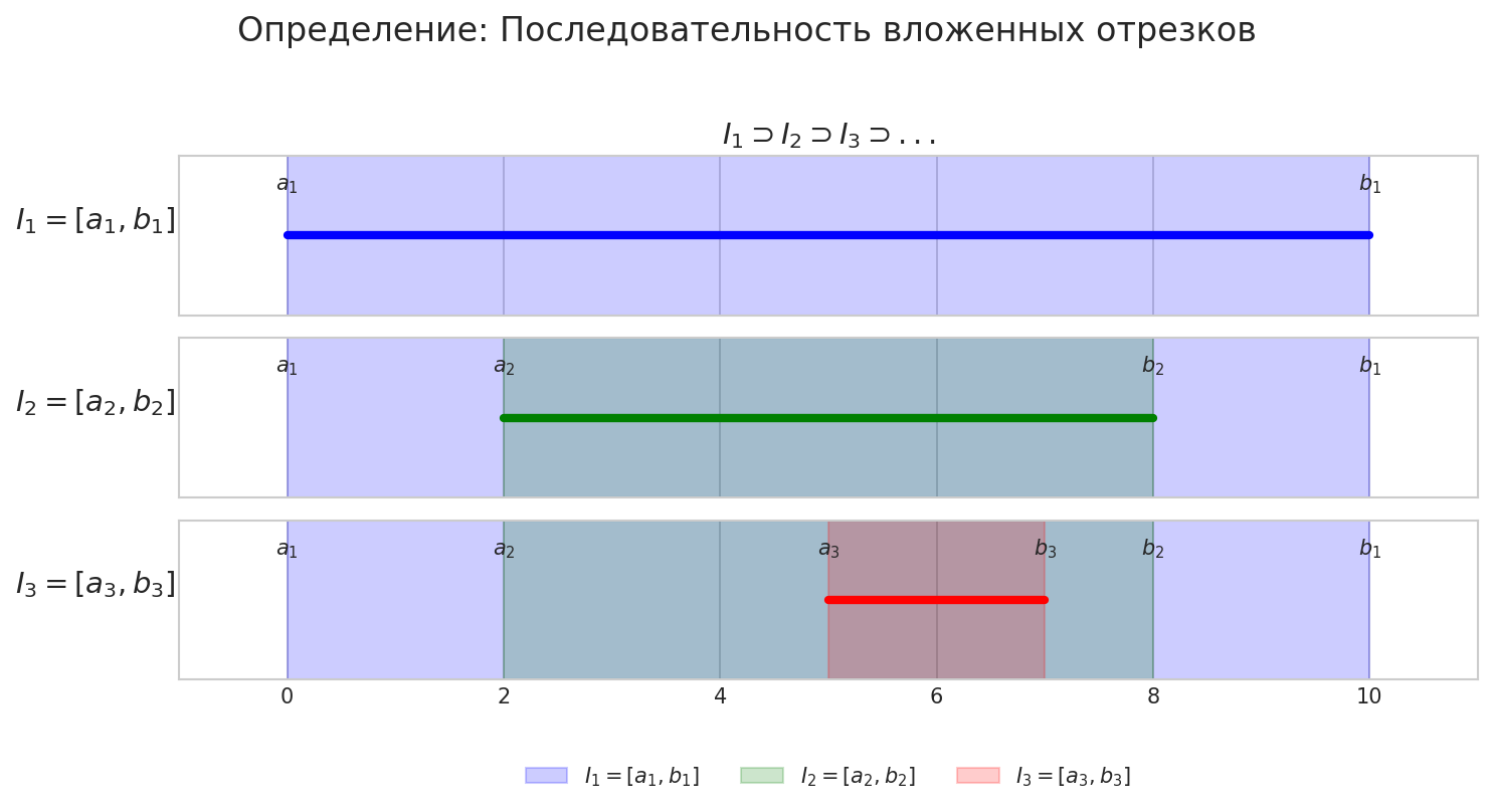
- Cantor's form: Every nested sequence of closed intervals shares at least one common point.
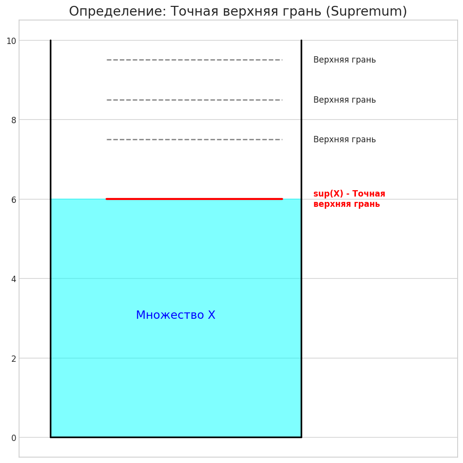
- Weierstrass's form: Every nonempty set bounded above possesses a least upper bound (supremum).
Related concepts:
- Upper bound (majorant): any number ≥ all elements of the set
- Supremum (least upper bound): the minimal upper bound
- Infimum (greatest lower bound): the maximal lower bound
Without the completeness axiom, limits and derivatives would collapse. It is the foundation upon which all of analysis is built.
Chapter 8. Why You Cannot Count All Points on a Line
Can we enumerate all real numbers on [0, 1] as a complete list: x1, x2, x3, ...?
Cantor's Diagonal Method:
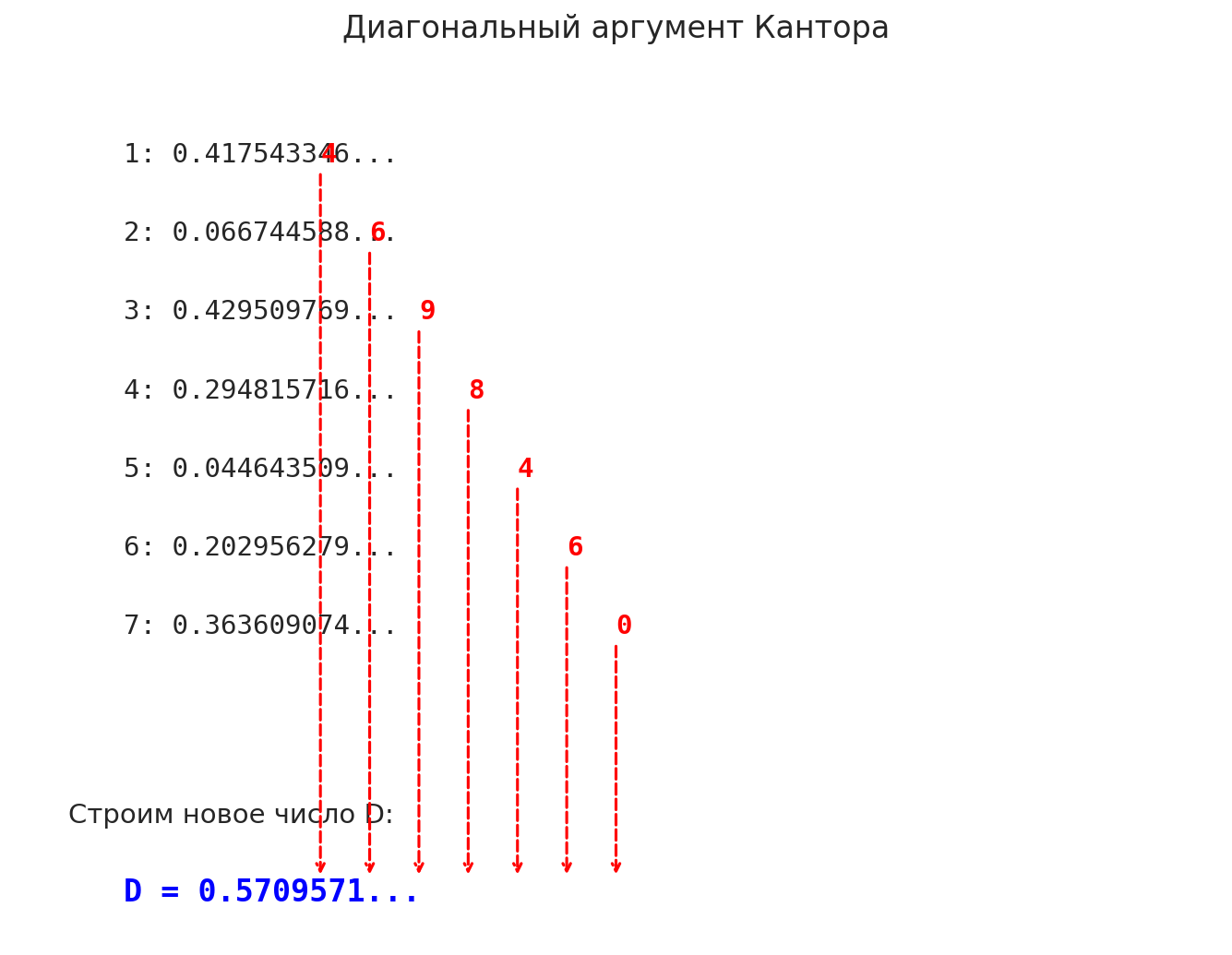
Suppose someone claims to possess a complete enumeration of all real numbers in [0, 1]. We construct a counterexample D (the diagonal number) by:
- Taking the 1st decimal digit of x1 and changing it.
- Taking the 2nd decimal digit of x2 and changing it.
- Taking the nth decimal digit of xn and changing it.
This new number D differs from every listed number at position n (from xn). Therefore, D exists in [0, 1] but isn't in the "complete" list — a contradiction.
But there is also a more elegant approach...
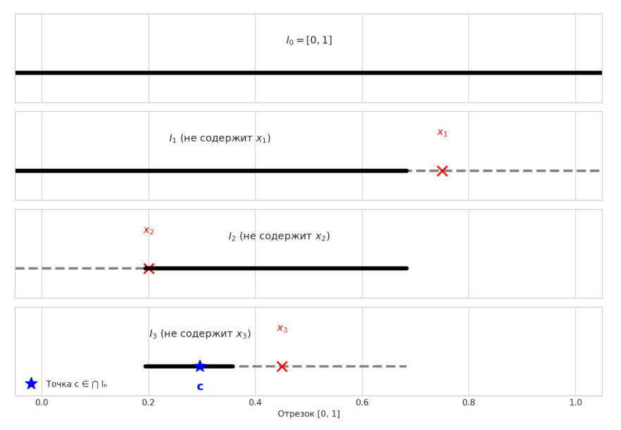
The Nested Intervals Proof:
Rather than manipulating digits, we use geometric intuition:
- For any claimed enumeration, divide [0, 1] into three parts; choose interval I1 that avoids x1.
- Subdivide I1 and choose I2 that avoids x2.
- Continue indefinitely: I0 ⊃ I1 ⊃ I2 ⊃ I3 ⊃ ...
By the axiom of completeness (Cantor's form), the intersection of all these nested intervals contains at least one point c.
The trap: Point c must exist in [0, 1]. But by construction:
- c cannot equal x1 (it's not in I1)
- c cannot equal x2 (it's not in I2)
- c cannot equal xn for any n (it's not in In)
Thus c wasn't in the original list, proving any enumeration is incomplete.
The cardinality hierarchy:
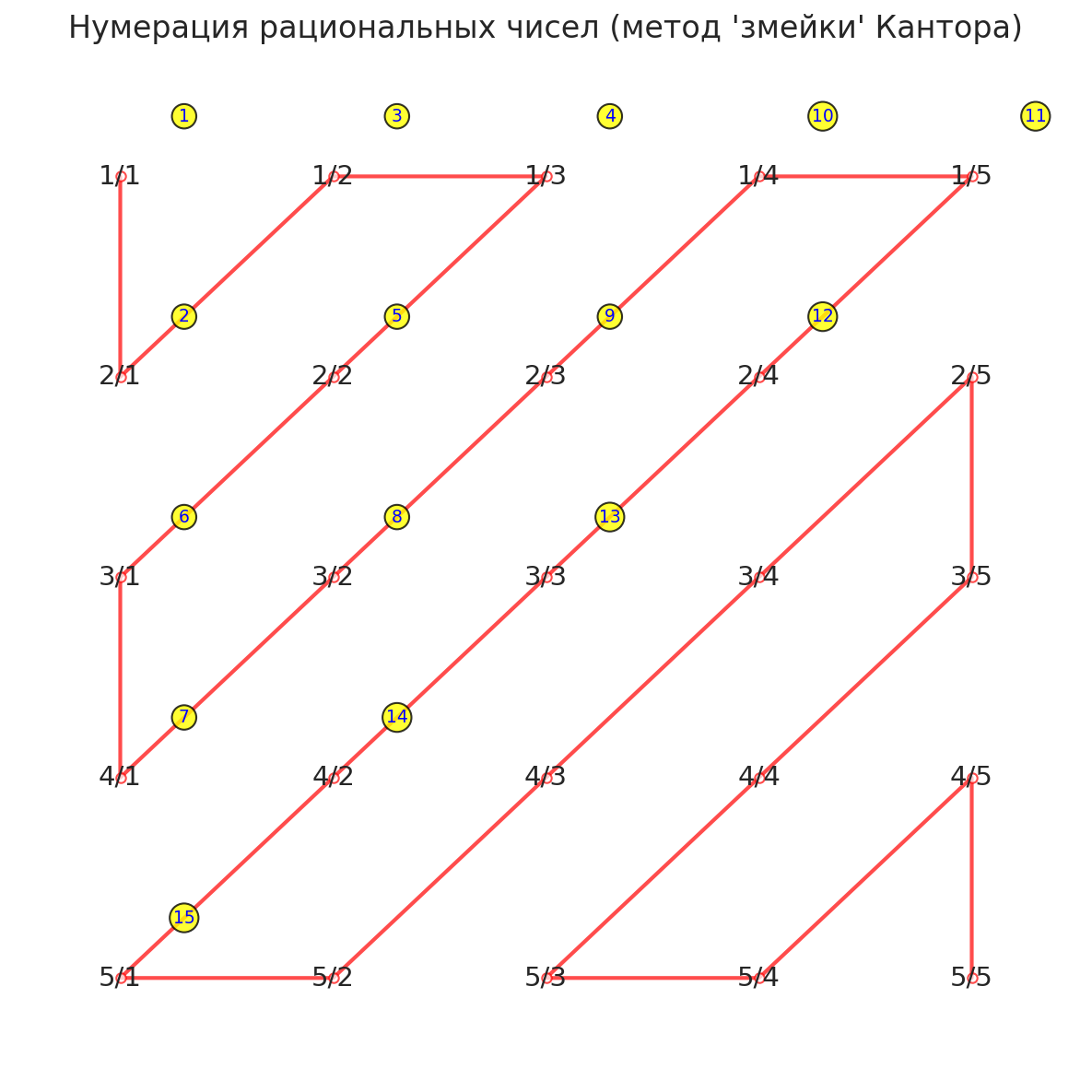
- ℕ (naturals) and ℚ (rationals) are countable — they match in "quantity" despite ℚ being denser.
- ℝ (reals) is uncountable — strictly larger in cardinality.
Uncountability is not abstract mathematics — it mathematically expresses the "solidity" and "seamlessness" that Aristotle sought in continuity. The fact that real numbers cannot be listed reveals why they form a true continuum.
Chapter 9. The Beauty of Simplicity: How to Prove the Same Thing More Elegantly
The nested-intervals proof exemplifies how the same mathematical truth can be expressed through different languages — combinatorial (Cantor's diagonal) versus topological (interval nesting).
Why does the nested intervals method surpass the diagonal?
- It doesn't depend on any particular number system (decimal, binary, etc.).
- It directly appeals to connectedness and completeness properties.
- It visualizes an infinitely shrinking "refuge" that guarantees at least one escape point.
The geometric insight: as intervals narrow infinitely, the axiom of completeness guarantees the survival of at least one point. This represents a topological victory rather than a computational one. The beauty lies in how topology — the study of continuity and closedness — supplants mere digit arithmetic.
This proof demonstrates that mathematical rigor need not require algebraic manipulation. Instead, it flows from:
- A clear geometric setup (the interval sequence)
- An axiomatic foundation (completeness)
- Logical inference (contradiction in assuming completeness fails)
The nested-intervals method preserves intuition while maintaining full rigor. Students see why the real line cannot have a complete enumeration: there is always "room" for undiscovered points in the ever-tightening gaps. This visual-logical harmony represents analysis at its finest.
Part III. Building Proper Analysis: Without Epsilon-Delta
Chapter 10. Building the Foundation: Axioms, Definitions, and Theorems
Now we have all the ingredients to build analysis properly. Real numbers ℝ are characterized by three groups of axioms:
- Field axioms — standard arithmetic operations and their properties (commutativity, associativity, distributivity, existence of identity elements and inverses).
- Order axioms — comparison relationships and their consistency (trichotomy, transitivity, compatibility with operations).
- The Completeness axiom — the crown jewel that distinguishes ℝ from ℚ, formulated in three equivalent ways: Dedekind cuts, Cantor's nested intervals, and Weierstrass's least upper bound.
With these axioms in hand, we can define the key concepts without quantifiers:
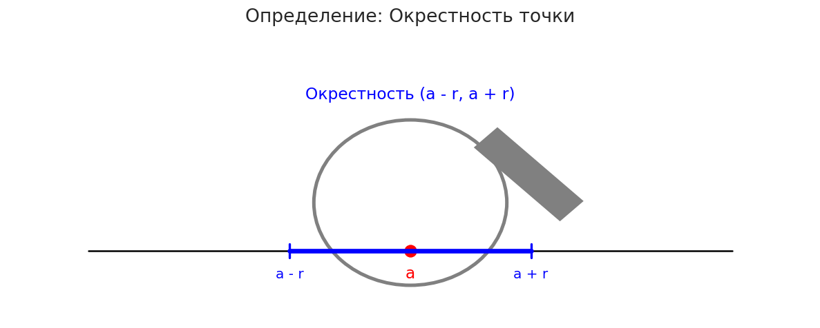
Neighborhood of point a with radius r: the interval (a − r, a + r). A symmetric window around the point.
Accumulation point: A number a is an accumulation point of sequence {xn} if every neighborhood of a — no matter how small — contains infinitely many elements of the sequence.
Sequence convergence: A sequence converges to limit a if a is the unique accumulation point AND only finitely many terms lie outside any neighborhood of a.
Now three fundamental theorems follow naturally:
Theorem 1 — Convergent sequences are bounded.
Proof: The accumulation point is surrounded by infinitely many terms in any neighborhood. The remaining finitely many terms fit in a larger interval. Combining both regions gives a bound for the entire sequence.
Theorem 2 — Bolzano-Weierstrass Theorem.
Every bounded sequence contains a convergent subsequence. This follows because the completeness axiom guarantees that accumulation points must exist — the terms of a bounded sequence cannot escape entirely from a closed interval.
Theorem 3 — Monotone Bounded Sequences Converge.
A monotone sequence cannot have multiple accumulation points. Once it moves past one accumulation point, it can never return — this creates a contradiction. Therefore, it has exactly one accumulation point and converges.
Continuous Functions
Definition (Heine): A function f is continuous at point c if for any sequence {xn} converging to c, the sequence {f(xn)} converges to f(c).
In other words: the limit of the function equals the function of the limit. No epsilon-delta machinery required.
Weierstrass's Theorem on Compact Sets: A continuous function on a closed interval [a, b] is bounded and attains its maximum and minimum values. The proof elegantly uses Bolzano-Weierstrass: if values were unbounded, extract a convergent subsequence of arguments and derive a contradiction with continuity.
Chapter 11. What's Next? Analysis Without Suffering, and Little-o
Traditional approaches require mastery of nested quantifiers (∀ε ∃δ...) as an entry barrier, alienating students from the underlying geometric meaning. There is a better way.
Little-o Notation: o(h)
Definition: A function α(h) = o(h) means that limh→0 α(h)/h = 0.
Geometric meaning: these are functions that vanish faster than h itself — a notation for "negligible corrections."
Five algebraic properties of little-o:
- Absorption: o(h) + o(h) = o(h)
- Scaling: C · o(h) = o(h) for any constant C
- Power reduction: h · o(h) = o(h²)
- Hierarchical dominance: o(h³) ⊂ o(h²) ⊂ o(h)
- Product rule: o(hn) · o(hm) = o(hn+m)
These properties transform limit proofs into algebraic calculations, eliminating epsilon-delta machinery while maintaining full rigor.
The Derivative Redefined:
Traditional: f′(x) = limh→0 [f(x + h) − f(x)] / h
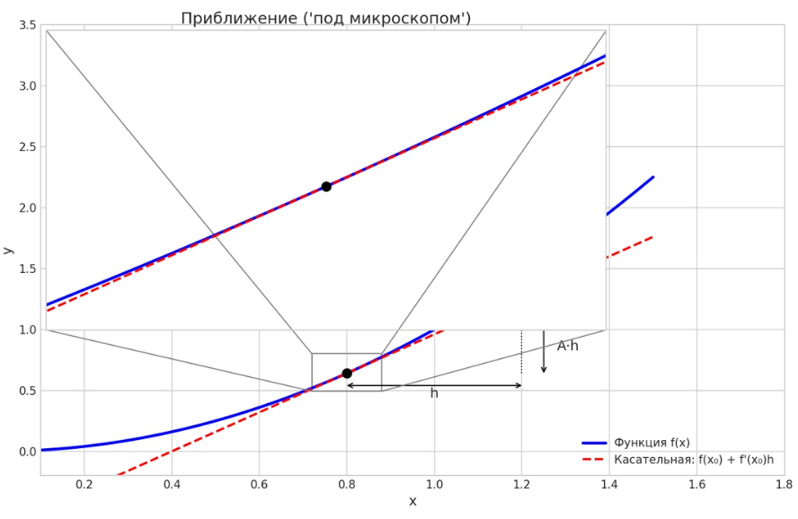
Via little-o: f(x0 + h) − f(x0) = A · h + o(h), where A = f′(x0).
This reformulation reveals the derivative as the best linear approximation — not just a limit formula but a geometric statement about tangent lines.
Roadmap for the rest of analysis:
- Local behavior theorems follow immediately from linear approximations.
- Rolle's Theorem: a foundation built using Weierstrass's theorem on extrema.
- Mean Value Theorems: geometric rotations of Rolle's theorem.
- Taylor's Formula: a natural refinement, adding higher-order terms beyond the linear approximation.
- Integration, series, multivariate functions: structural parallels using norms and Jacobian matrices extend the same ideas to higher dimensions.
Epilogue. The Great Deception: Why Analysis Is Geometry, Not Algebra
The "rigor crisis" of 19th-century mathematics prioritized arithmetic formalization over geometric intuition. Cauchy's epsilon-delta approach satisfied this agenda perfectly — it was purely numerical, avoiding visual representation entirely.
The irony: by the 20th century, geometry itself gained rigorous axiomatization through Hilbert systems and vector calculus. This proved that formalization and intuition were never mutually exclusive. The choice of epsilon-delta was not inevitable — it was historical accident.
The core deception is presenting the formalization language (algebraic inequality manipulation) as the essence rather than mere notation of analysis:
| Concept | Geometric Reality | Algebraic Disguise |
|---|---|---|
| Limit | Spatial proximity | ε-δ inequalities |
| Derivative | Tangent line | Limit formula |
| Integral | Area under curve | Riemann sum limits |
The metaphor: explaining paintings exclusively through RGB pixel codes provides complete technical information while destroying understanding. The epsilon-delta formalism does the same to analysis.
Addressing "pathological" counterexamples:
Weierstrass's nowhere-differentiable continuous function is not a failure of geometric thinking but its triumph. Its construction is purely geometric: repeatedly overlay increasingly fine zigzags. The result is a fractal — an infinitely intricate geometric structure.
"Monsters" like the Cantor function reveal the richness of the continuum, not its bankruptcy. Hiding this beauty behind algebraic machinery impoverishes mathematical pedagogy.
The false dichotomy:
Descartes united algebra and geometry: use algebra to answer geometric questions. Modern analysis inverts this relationship — treating algebra as master and geometry as servant. The author advocates restoring geometry to its rightful foundational role.
By replacing ∀ε ∃δ with "point clustering" and o(h) with "negligible terms," we demonstrate that Heine's sequential approach provides equal rigor with vastly superior pedagogy. This challenges the universally accepted Cauchy-Weierstrass formalism that has dominated for 150 years.
The essence of analysis is geometry and topology — the study of how space behaves. The symbols are merely notation. Understanding this distinction is the first step toward genuinely learning calculus.