"Hello! I Am [0.44, -0.91, 0.66...]" — How to Teach a Machine to Understand the Meaning of Words

Introduction

Machine learning models can analyze text to detect spam or determine sentiment in movie reviews. They understand that "pear" relates more closely to "apple" than to "steamship." The foundational principle behind all of this is converting input data into numbers — images, text, audio, and video files all become numerical representations before a model can work with them.

To feed objects into ML models as concepts, we transform them into numerical sets that help distinguish whether something is an "apple" versus a "pear." Grayscale images use pixel values from 0 (darkest) to 1 (brightest), simplifying processing and allowing neural networks to learn from these values.

The big challenge is: how do we convert letters and words into numbers?

Attempt #1: Simple Numbering

The most straightforward approach assigns a unique number to every unique word through tokenization. Each word gets a unique index number.

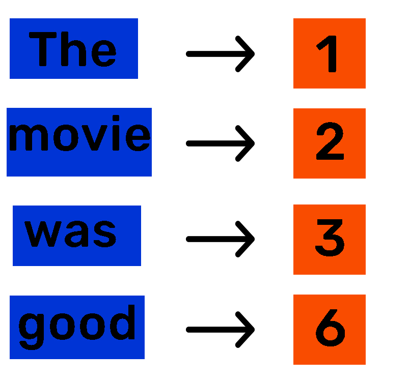
This seems like a solved problem — we have numbers the model can accept. But this method is only suitable for ordinal features where numbers imply a ranking.

Consider these three sentences:

1. "The movie was good."
2. "The movie was bad."
3. "The movie was awesome."

Suppose we assign: good=6, bad=26, awesome=27. The numbers 26 and 27 are close to each other, which might suggest to the model that "bad" and "awesome" are similar — when in reality "good" and "awesome" share meaning. This false proximity causes models to misinterpret relationships and make incorrect predictions.

Attempt #2: One-Hot Encoding

One-Hot Encoding solves the false proximity problem by representing each word with a unique vector sized to the vocabulary length.

For a vocabulary of [The, movie, was, good, bad, awesome] = 6 words:

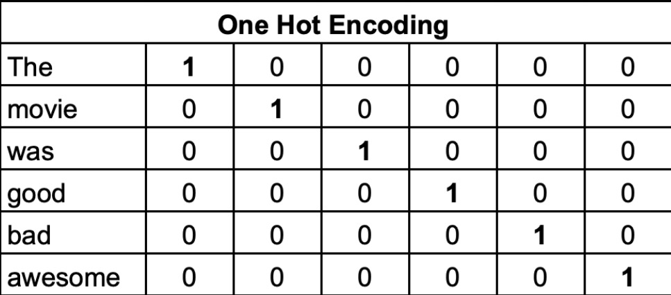
Each word gets a unique vector with a single "1" (indicating its presence) and all other positions as "0". This eliminates ranking problems and treats all words equally without hidden numerical relationships.

Limitations: One-Hot Encoding creates sparse vectors. A 20,000-word vocabulary produces 20,000-dimensional sparse vectors, demanding significant memory and computational resources. Additionally, it completely lacks semantic and contextual meaning — it treats words as entirely independent entities without capturing the fact that "good" and "awesome" are conceptually similar. These constraints make One-Hot Encoding inefficient for large-scale natural language processing tasks.

Attempt #3: Bag of Words and N-grams

Bag of Words simply counts word occurrences in sentences.

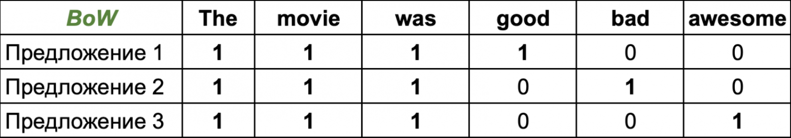
Since individual words are processed independently, this is called a unigram approach. Using two-word combinations (bigrams) captures more context than One-Hot Encoding, while N-grams extend this to N-word sliding windows.

Challenges: Large datasets generate enormous numbers of N-gram combinations, creating massive sparse feature vectors that require excessive memory. Since models can only consider a limited number of consecutive words in order, N-grams fail to capture deeper meanings or relationships between distant words. For example, in "The librarian was looking for a book," the words "librarian" and "book" are not adjacent, so N-grams miss their obvious semantic connection.

Attempt #4: Semantics and Context

An effective model must understand both semantics (word meaning) and context (surrounding environment).

Consider this text:

"Mechanic Bogdan entered the noisy garage, wiping oil from his nine-millimeter wrench, approached the workbench and grabbed his large heavy..."

To predict the next word, the model needs semantic understanding of each word and the sentence context. Humans immediately recognize: Where is the mechanic? In a garage/workshop. Does "heavy" describe the mechanic or the object? The sentence structure clearly shows "large" and "heavy" describe something being picked up, not the person.

The context mentions "workbench" and "grabbed." We infer the object is a work tool. Semantically, replacing "mechanic" with "master" or "garage" with "auto shop" should preserve meaning without drastically changing predictions. We would expect "hammer," "wrench," or "tool" — objects that are typically heavy, located on workbenches, and used by mechanics.

To train models that understand semantic and contextual meaning, we encode training data into feature vectors that capture both aspects. This is where Word Embeddings and attention mechanisms become essential.

What Are Word Embeddings?

A Word Embedding represents words as dense numerical vectors in continuous n-dimensional space. Each word receives a fixed-dimension vector — unlike One-Hot Encoding where most values are zero. Similar vectors correspond to similar words, and directional meaning exists in vector space.

A two-dimensional example: "coffee" and "tea" vectors cluster closer together than to unrelated words like "brick."

Consider a one-dimensional example: a number line representing animal size, encoding ten animals where similar-sized animals cluster together. Expanding to two dimensions (X = size, Y = danger): "tiger" and "lion" appear close (large, dangerous), while "cow" (large, safe) and "hamster" (small, safe) occupy different regions.

With semantically encoded vectors, mathematical operations become meaningful:

V(Son) - V(Man) + V(Woman) ≈ V(Daughter)

Subtracting "man" from "son" and adding "woman" yields a vector near "daughter" — showing that the difference between son/daughter mirrors the difference between man/woman.

V(Madrid) + V(Germany) - V(Spain) ≈ V(Berlin)

Madrid (Spain's capital) plus Germany minus Spain yields Berlin (Germany's capital) — because removing Spain's attributes and adding Germany's creates a result matching Berlin.

We cannot explicitly determine embedding space features or define them manually — they depend entirely on training data. Models capture semantic text understanding and represent it in a lower-dimensional vector space (hundreds or thousands of dimensions versus hundreds of thousands for large-vocabulary One-Hot Encoding).

Dense vectors store word values in n-dimensional embedding space. While high-dimensional embeddings cannot be directly visualized, mathematical tools like Principal Component Analysis (PCA) can project them into fewer dimensions for visualization.

In trained Word2Vec models, vectors associated with "coffee" include tea, sugar, cheese, and others — words frequently appearing in similar contexts.

How Embeddings Are Created

Word2Vec, introduced by Google, demonstrates two key techniques: Continuous Bag of Words (CBOW) and Skip-Gram.

CBOW (Continuous Bag of Words)

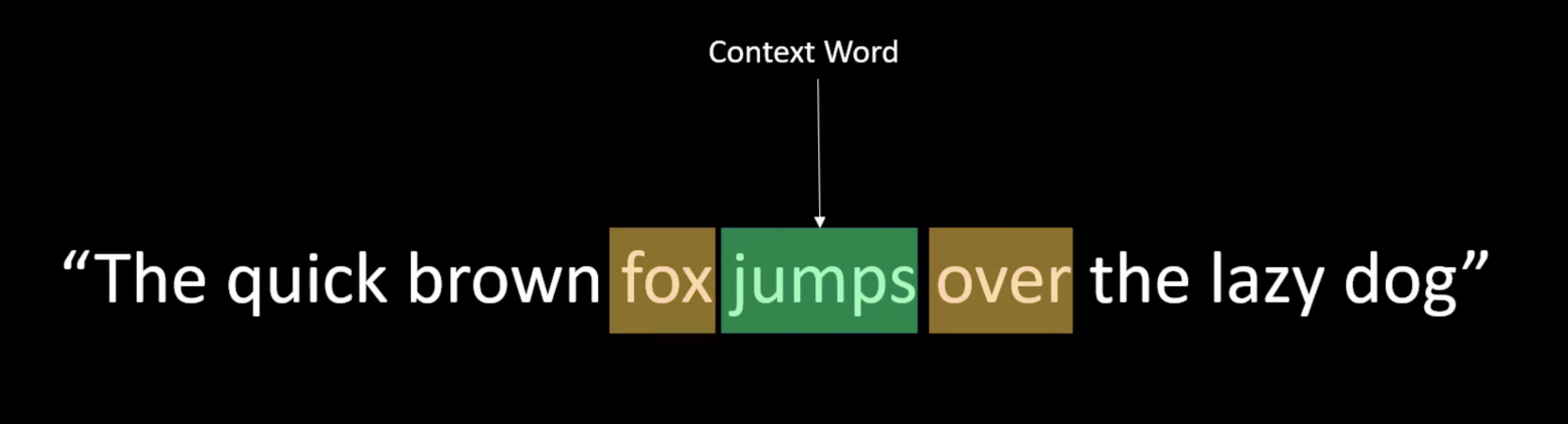
In CBOW, we take a context word window and predict the central target word from its neighbors.

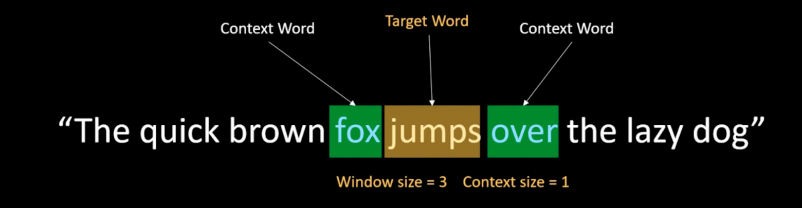
Given the input words "Fox" and "over," the target word might be "jumps." The model is a simple neural network.

Before loading data into the model, we apply One-Hot Encoding:

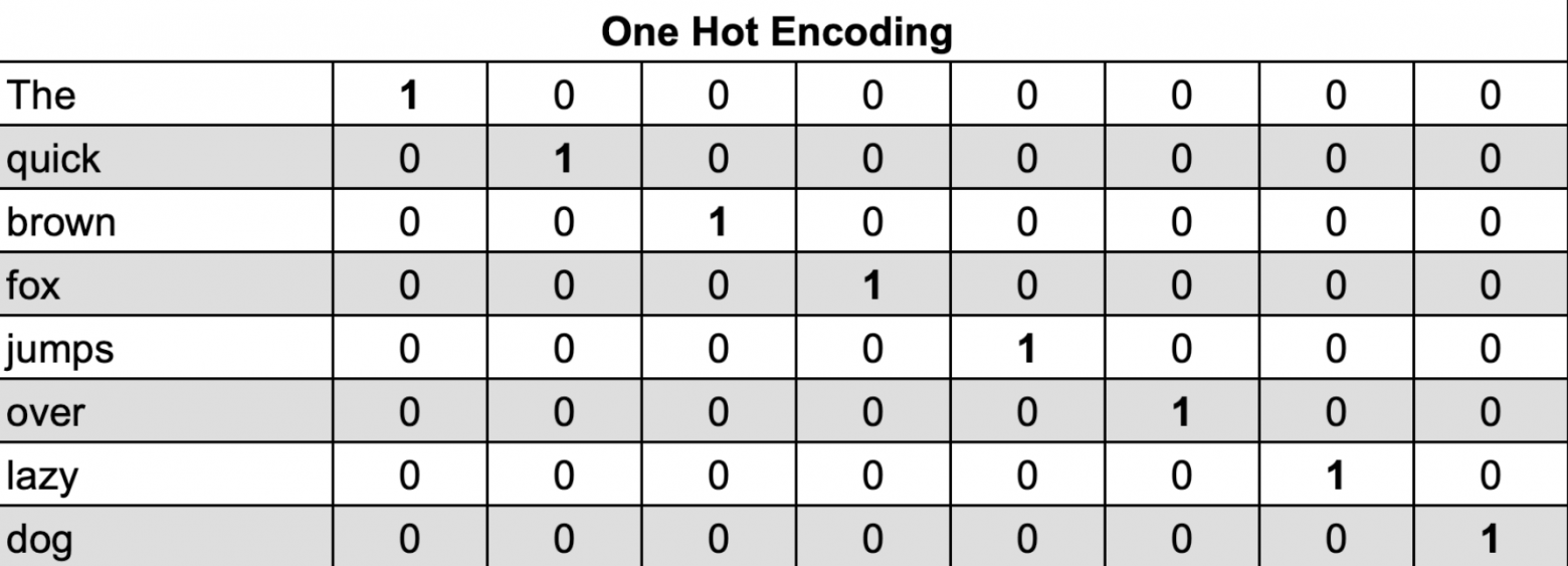
The input layer receives One-Hot Encoded vectors of context words. The hidden layer contains neurons equal to the desired embedding dimensionality.

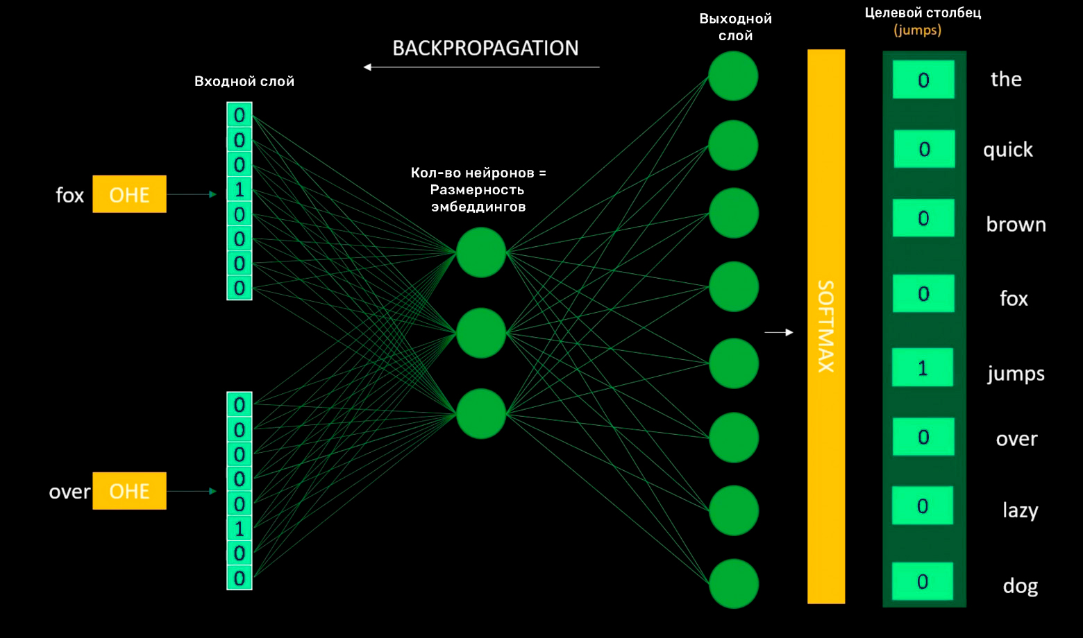
The output layer contains neurons equal to the vocabulary size. The weights between the output and hidden layers become the embedding matrix.

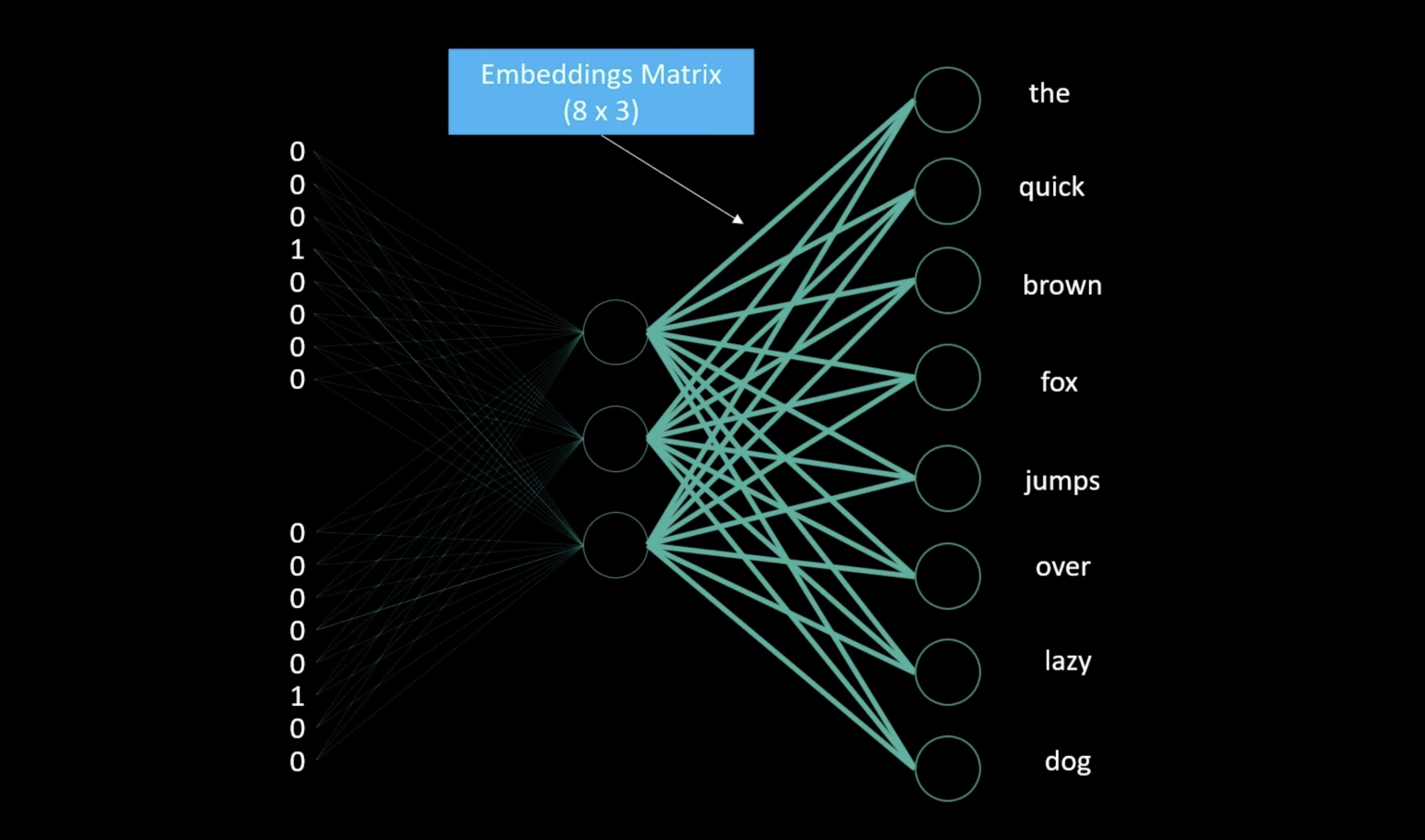
An 8x3 embedding matrix becomes a lookup table for each word. After training, this matrix provides three-dimensional vectors for each word with fixed individual representations. Since we trained on eight words, the embedding matrix is 8x3. Rows equal unique words (vocabulary size); columns equal the chosen embedding dimensionality.

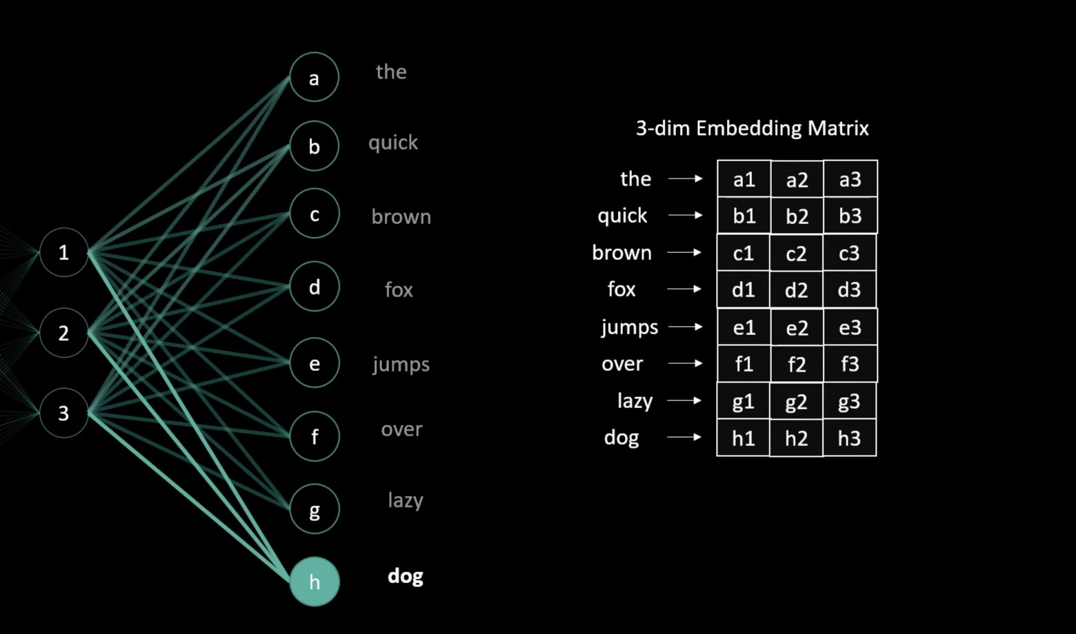
To obtain the embedding values for each word, convert the word to its one-hot vector, then compute the dot product with the embedding matrix to get the word's embedding vector.

Skip-Gram

Understanding CBOW makes Skip-Gram simple. Skip-Gram reverses the process: given a central word, predict the surrounding context words instead of predicting the central word from context.

Both methods work well for training word embeddings.

Embeddings in Transformer Architecture

Modern architectures like GPT and BERT modify this approach. The embedding layer is not necessarily pre-trained from Word2Vec but instead forms part of the model, trained from scratch or fine-tuned for specific tasks — primarily predicting the next token.

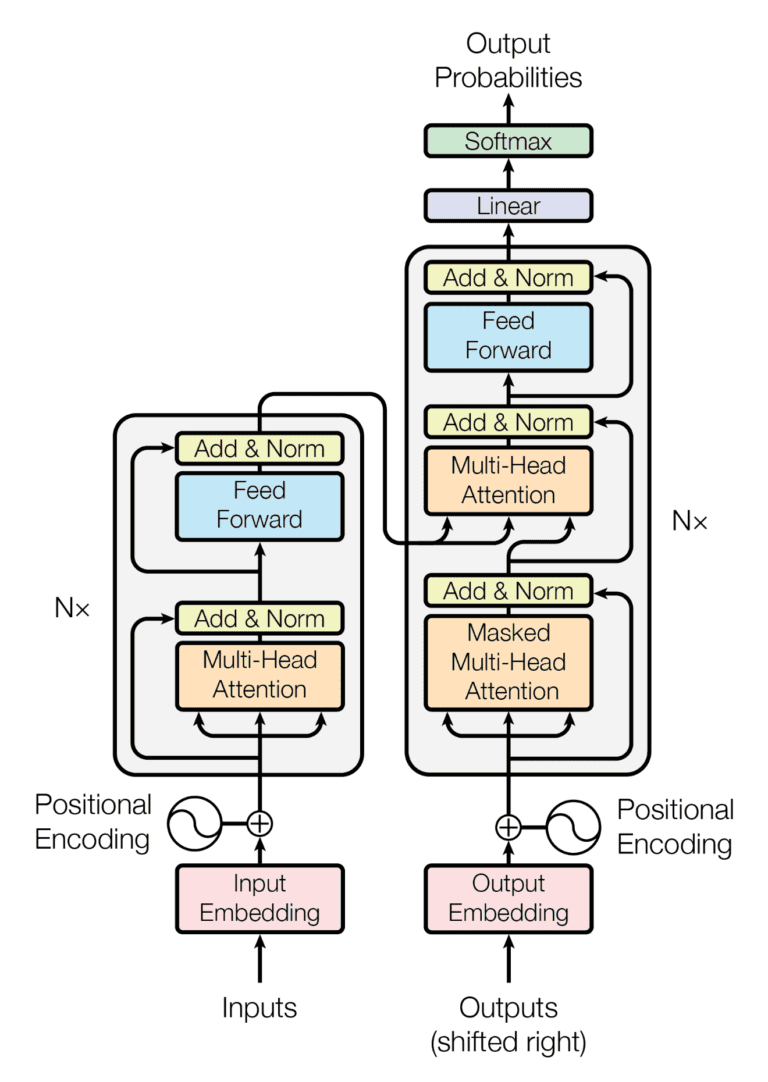
Looking at the decoder section of the Transformer:

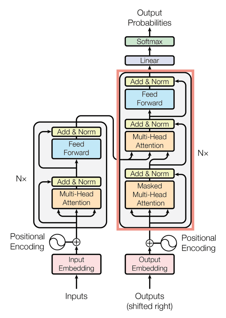
First, we convert text to tokens:

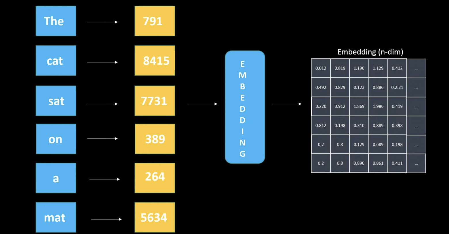
Six tokens yield an embedding matrix sized 6 x embedding dimensionality. The decoder layer doesn't use Word2Vec models but rather simple shallow neural networks to create embeddings.

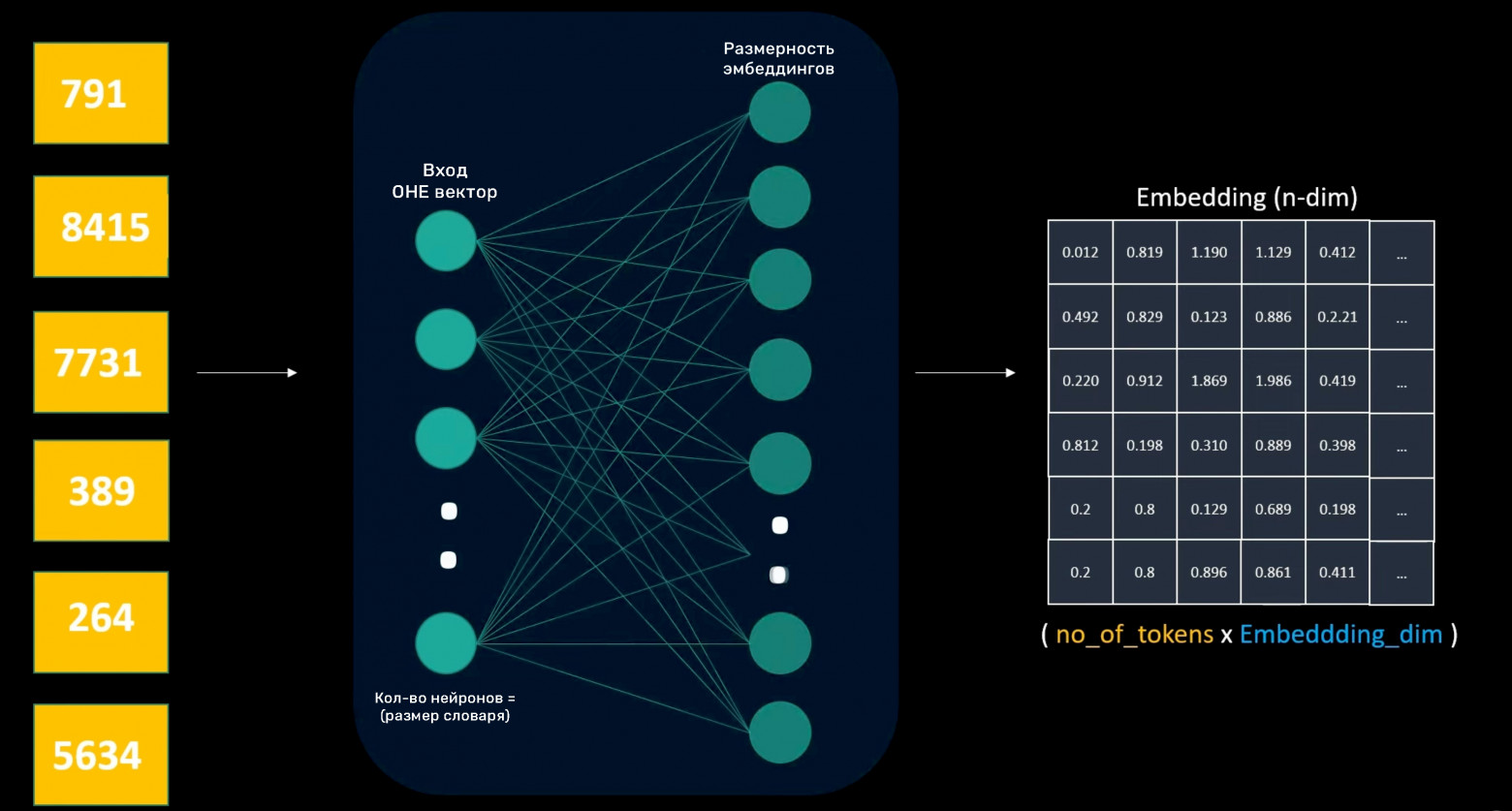
The input layer receives one-hot encoded word vectors. The neuron count equals vocabulary size; hidden layer neurons equal the desired embedding dimensionality.

Embedding layer weights are trainable parameters that learn n-dimensional word representations. Like Word2Vec, the weights function as a token lookup table where each token receives trained weight values. After text-to-token conversion, the embedding layer provides vector representations for each token. Properly trained embeddings capture semantic word meaning.

Unlike Word2Vec, where embeddings are trained separately, decoder-layer embeddings train alongside the entire model. Since our decoder predicts the next token, we use a special embedding layer that outputs vector representations of the input text. This embedding passes through repeated decoder blocks, eventually reaching the output layer that predicts the next token. The model calculates the error and performs backpropagation through all layers using training data.

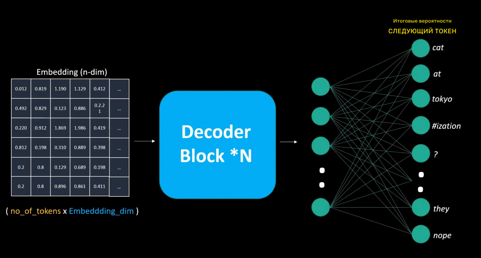
The output layer is similar to the initial embedding layer but inverted: instead of output size equaling the embedding dimensionality, it has neurons equaling the total vocabulary size, enabling probability assignment to every possible next token.

This process shows that models first represent tokens in n-dimensional embedding space, then use this representation for next-token prediction. Unlike Word2Vec (which predicts central words from context), large language models aim to predict the next word considering all previous words, with multiple decoder layers additionally processing embeddings before generating the next token.

Positional Encoding

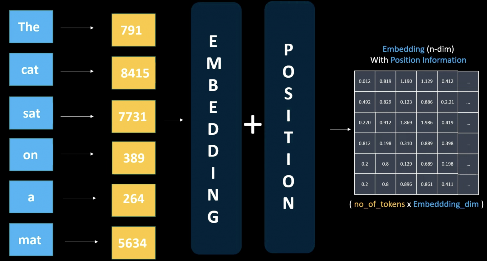
Unlike RNNs, which process each token individually and sequentially, Transformers process all words in parallel. We must inform the model of each token's position — which token comes first, which follows.

After embedding creation, we add a positional vector to the embedding vector, encoding each token's position information. Positional information can be either another trainable layer or a static numerical representation unique to each token. We simply add this positional vector to the embedding vector, creating a new representation containing both word meaning and position information. Importantly, the embedding matrix shape doesn't change — only the values shift slightly depending on token position.

This matrix is now ready for the attention mechanism — the first decoder block layer. Embedding layers capture semantic word meaning but don't provide contextual text understanding. Here, the attention mechanism plays a crucial role.

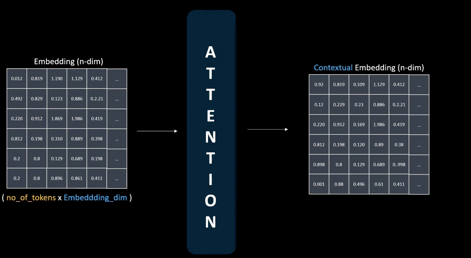
The attention mechanism is the heart of large language models, enabling them to capture word relationships beyond independent meanings. After passing through the attention mechanism, we obtain a contextual token representation that differs from the initial semantic representation. For instance, "wrench" (the tool) and "wrench" (to injure) carry identical spellings but semantically different meanings — the attention mechanism resolves this ambiguity based on context.

Conclusion

Combining simple solutions like tokenization and word counting gradually leads us toward Transformers and attention mechanisms. Today, embeddings appear everywhere — in recommendation systems, similar image searches, and fundamentally in ChatGPT and other large language models.

Understanding how CBOW, Skip-Gram, and Transformers work forms the foundation for deep exploration of natural language processing.

Thank you for reading!