Inventing JPEG

As you correctly understood from the title, this is not your typical description of the JPEG algorithm (I described the file format in detail in the article "Decoding JPEG for Dummies"). First and foremost, the chosen approach assumes we know nothing — not only about JPEG, but also about the Fourier transform and Huffman coding. And in general, we barely remember anything from our lectures. We simply took an image and started thinking about how we could compress it. So I tried to express only the essence in an accessible way, while giving the reader a sufficiently deep and, most importantly, intuitive understanding of the algorithm.

Knowledge of the JPEG algorithm is very useful beyond just image compression. It employs theory from digital signal processing, mathematical analysis, linear algebra, and information theory — in particular, the Fourier transform, lossless coding, and more.

If you're interested, I suggest going through the same steps on your own alongside this article. Check how well the reasoning applies to different images, try to make your own modifications to the algorithm.

Warning, heavy traffic! Lots of illustrations, graphs, and animations (~10MB). Ironically, in an article about JPEG, there are only 2 images in JPEG format out of about fifty.

Vector Representation

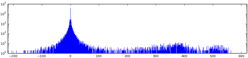
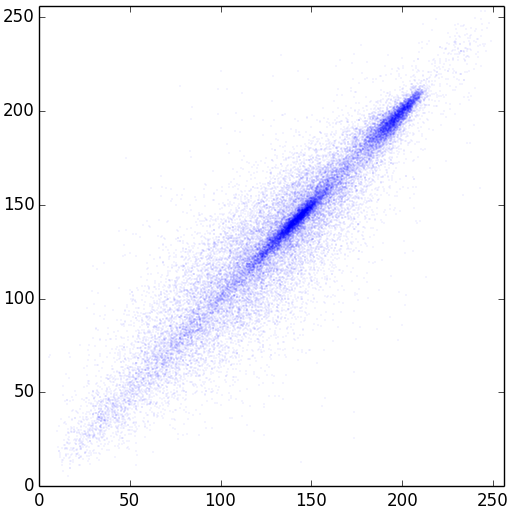
To verify the dependence of neighboring pixels, let's build a graph where each pair of pixels is marked as a point. Along the X axis — the value of the first pixel, along the Y axis — the second. For a 256x256 image, we get 32,768 points.

Most points lie close to the diagonal y=x, indicating strong correlation between neighboring pixels. This is the key property we'll exploit for compression.

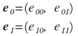
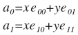
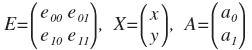
The solution: rotate the points by 45 degrees, transitioning to a new coordinate system with basis vectors e₀ and e₁. The vectors must be orthonormal (normalized by dividing by √2).

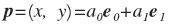
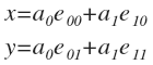
In the new system, any point p = (x, y) is represented as (a₀, a₁), where:

• a₀ — the average of x and y
• a₁ — their difference (normalized)

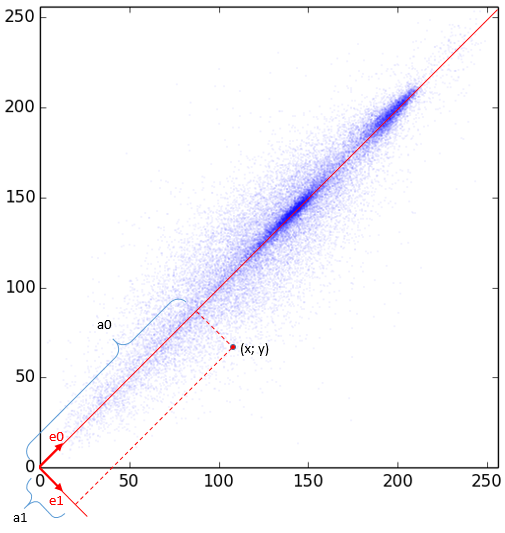
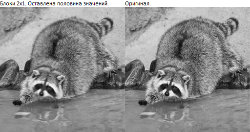
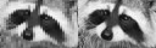
First experiment: If we keep only a₀ (setting a₁ to zero) and reconstruct the image, we get a heavily blurred version. The quality is unsatisfactory, although the data volume is halved.

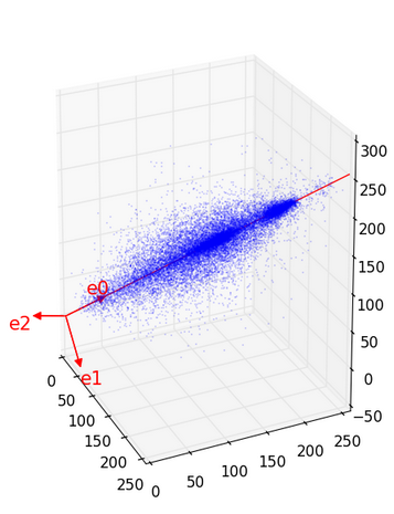
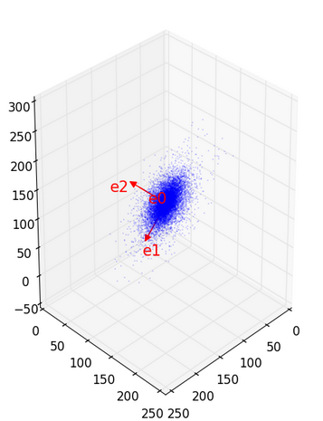
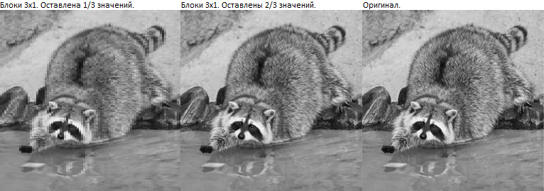
Extending the idea: Let's divide the image into triples of pixels and represent them as three-dimensional vectors. The red axes on the 3D graph indicate the optimal basis directions e₀, e₁, e₂.

Results when discarding a₂:

• The second image looks significantly better
• Sharp transitions are smoothed, but structure is preserved
• Data is reduced by one third

Key conclusion: We need to find a way to transform a sequence (x₀, x₁, ..., xₙ₋₁) into (a₀, a₁, ..., aₙ₋₁) such that each aᵢ becomes progressively less important than the previous ones. This requires a mathematical approach to finding the optimal basis.

Transitioning from Vectors to Functions

The author introduces the concept of discrete functions as an alternative to working with N-dimensional vectors.

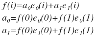
Example: For two pixels (x, y), we define a function f(i), where f(0)=x and f(1)=y. Based on the basis vectors, we create basis functions e₀(i) and e₁(i).

Fundamental observation: "Decomposing a vector into orthonormal vectors" is equivalent to "decomposing a function into orthonormal functions." The difference is only in formulation — the mathematics remains identical.

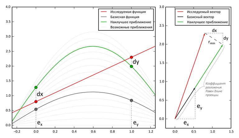
The decomposition process:

• The function is represented as a sum of basis functions with coefficients
• Each coefficient is found through the dot product (projection)
• The result provides the best mean-square approximation

Connection to Fourier series: The reasoning described above applies to any orthogonal basis. A special case is the Fourier series expansion — a specific choice of basis from sinusoids and cosines.

Discrete Fourier Transforms

In the previous section, we concluded that it makes sense to decompose functions into component parts. In the early 19th century, Fourier studied heat distribution along a metal ring and discovered that temperature could be expressed as a sum of sinusoids with different periods.

Periodic functions and harmonics: It turned out that periodic functions decompose wonderfully into sums of sinusoids. In nature, there are many objects and processes described by periodic functions, making this a powerful analytical tool.

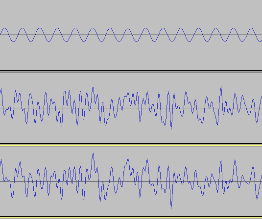
Sound is one of the most visual examples of periodic processes.

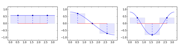
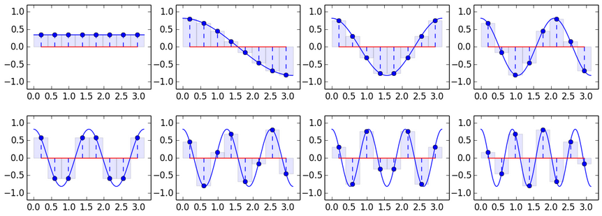
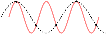
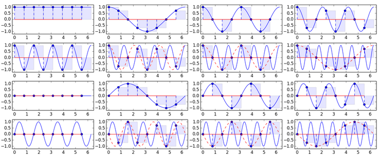
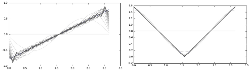
Why sinusoids as a basis? From the presented graphs, it becomes clear how to obtain eight basis vectors. Verification shows that these vectors are pairwise perpendicular (orthogonal), which allows using them as a basis.

DCT formula: "This is all the same formula: A = EX with the substituted basis." The basis vectors are orthogonal but not orthonormal.

Application to images: Despite the arguments for sinusoids, an image can be unpredictable even in small areas. Therefore, the picture is divided into small pieces. In JPEG, the image is cut into 8x8 squares. Within such a piece of a photograph, things are usually uniform, and such areas are well approximated by sinusoids.

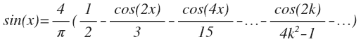
Gibbs effect: During decomposition, a problem arises — near sharp transitions, characteristic bands appear (the Gibbs effect).

"The height of these humps appearing near function discontinuities does not decrease as the number of summand functions increases." The effect only disappears when almost all coefficients are preserved.

Important note: A false impression may form that the first few coefficients are always sufficient. This is true for many areas, but at the boundary of contrasting regions, values change sharply, and even the last coefficients are large.

DCT vs. Everything Else

We investigated orthogonal transforms and searched for results on DCT's optimality on real images. "DCT is most commonly found in practical applications due to its 'energy compaction' property" — this property means the maximum amount of information is concentrated in the first coefficients.

A study was conducted using a bunch of different images and known bases to calculate the mean squared deviation.

Comparison results: If you look at the graphs of preserved energy versus the number of coefficients, DCT takes "third place" — it's surpassed by other transforms.

KLT

"All transforms except KLT are transforms with a constant basis." In KLT (Karhunen-Loeve Transform), the most optimal basis for several vectors is computed. The first coefficients give the smallest mean-square error summed across all vectors.

Although this sounds appealing, practical problems arise: the need to store the basis and high computational complexity. DCT loses only slightly, but fast transform algorithms exist for it.

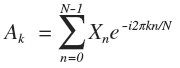
DFT

DFT (Discrete Fourier Transform) — the discrete Fourier transform.

One might think that a pure harmonic signal would give only one non-zero coefficient in DCT decomposition. This is incorrect — the phase of the signal also matters. For example, decomposing a sine wave using cosines yields many coefficients.

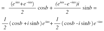
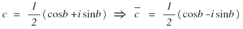
Using sines and cosines: It's more convenient to decompose into a sum of sines and cosines (without phases). Using Euler's formula, one can transition to complex form.

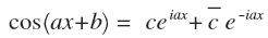
"DFT decomposes a signal into harmonics with frequencies from one to N oscillations." By the Nyquist-Shannon theorem, the sampling frequency must exceed the signal frequency by a factor of two.

DFT problems: The second half of complex amplitudes is a mirror image of the first. Harmonics have edge values equal to each other. Each is nearly mirror-symmetric about the center. This is bad for coding — compressed image block boundaries become visible.

An asymmetric signal is approximated inadequately — it requires harmonics closer to the end.

DST

"What if instead of cosines in DCT we use sines?" We'd get the Discrete Sine Transform. However, for image compression, this is inefficient since sines are close to zero at boundaries.

Returning to DCT

At the boundaries, DCT works well — there are counter-phases and no zeros.

Everything Else

Non-Fourier transforms:

• WHT — the matrix consists only of step functions with values -1 and 1
• Haar — an orthogonal wavelet transform

They are inferior to DCT but easier to compute.

Requirements for a new transform:

1. The basis must be orthogonal
2. It's impossible to surpass KLT in quality; DCT barely loses on real photographs
3. Using the example of DFT and DST, we must remember about boundaries
4. DCT's derivatives near boundaries equal zero, so the transition between blocks is smooth
5. Fourier transforms have fast algorithms O(N*log N)

"This section turned out like an advertisement for the Discrete Cosine Transform. But it really is awesome!"

Two-Dimensional Transforms

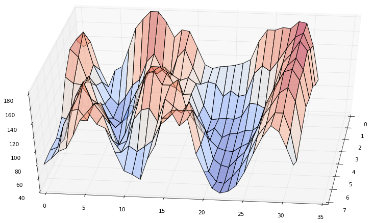
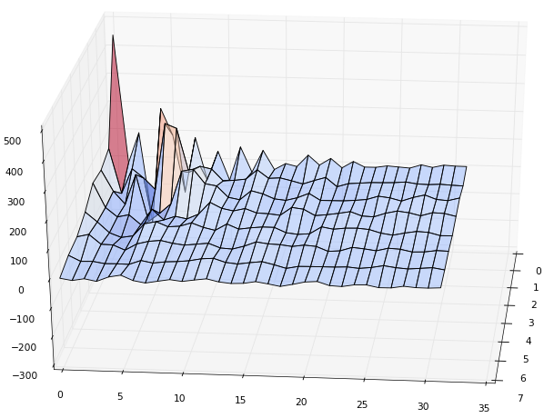
The experiment begins with a small piece of the image.

Applying by rows: We run DCT(N=32) across each row.

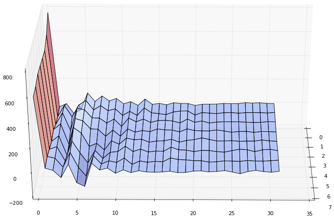
Applying by columns: "The values of each column of the resulting coefficients can be decomposed in exactly the same way as the original image values." DCT(N=8) is applied along columns.

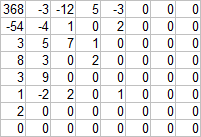
"Coefficient (0,0) turned out to be too large, so in the graph it's reduced by a factor of 4."

Result structure:

• Top-left corner — the most significant coefficients of the most significant coefficients' decomposition
• Bottom-left corner — the least significant coefficients of the most significant coefficients' decomposition
• Top-right corner — the most significant coefficients of the least significant coefficients' decomposition
• Bottom-right corner — the least significant of the least significant

Significance decreases diagonally from the top-left to the bottom-right corner.

Mathematical formula: By rows: A₀ = (Eᵀ)ᵀ = XEᵀ, then by columns: A = EA₀ = EXEᵀ.

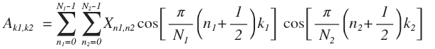
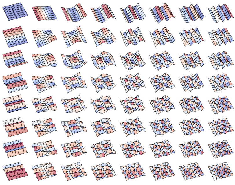
"Thus, if a vector decomposes into sinusoids, then a matrix decomposes into functions of the form cos(ax)*cos(by)." Each 8x8 block is represented as a sum of 64 functions.

Coefficient relationship: Coefficients (0,7) or (7,0) are equally useful.

"This is essentially ordinary one-dimensional decomposition onto 64 64-dimensional bases." Everything said applies not only to DCT but to any orthogonal decomposition. By analogy, one obtains N-dimensional orthogonal transforms.

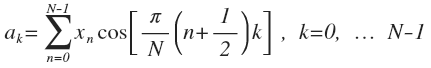
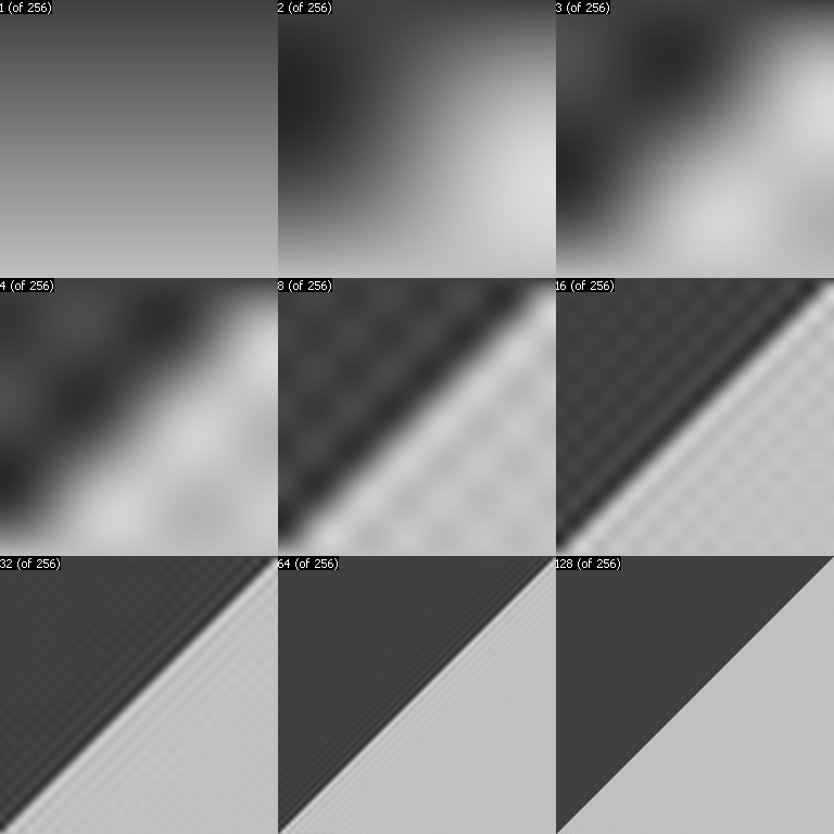
The numbers on the image indicate the count of non-zeroed coefficients (the most significant ones in the triangular region of the top-left corner are preserved).

Terminology: "Remember that coefficient (0,0) is called DC, the remaining 63 are called AC."

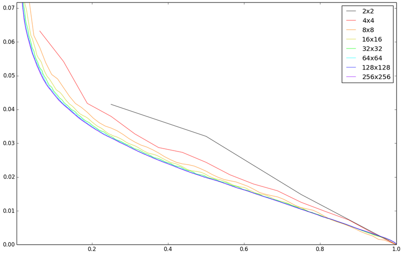
Block Size Selection

Why does JPEG use 8x8 blocks rather than larger or smaller ones?

A common claim states: "DCT works well only on periodic functions, and if you take 64x64 blocks, you'll likely need many high-frequency components." However, this reasoning applies to DFT rather than DCT.

Three main arguments against larger blocks:

1. Diminishing returns: Larger blocks offer minimal compression gains beyond 8x8
2. Computational complexity: Block size NxN requires O(N² log N) operations; doubling the size doubles complexity
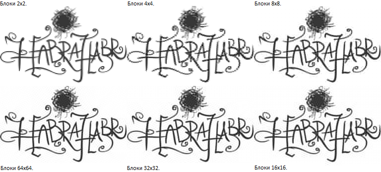
3. Gibbs effect: Larger blocks containing sharp boundaries produce visible artifacts

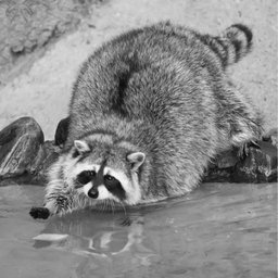
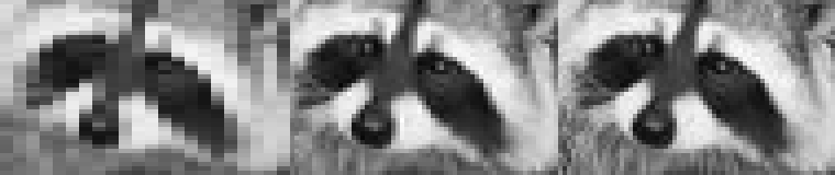
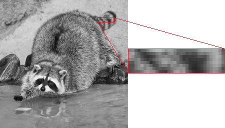
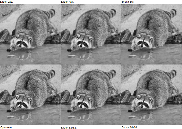
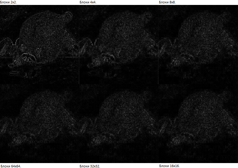
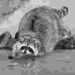
Experimental evidence comparing 4x4, 8x8, 16x16, and 32x32 blocks using the raccoon image demonstrates that 8x8 represents a reasonable balance between quality and processing speed.

Quantization

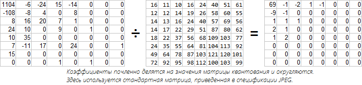
This section explains lossy compression through quantization matrices. Each DCT coefficient is divided by the corresponding matrix value, then rounded.

A standard JPEG quantization matrix is provided, with higher values for high-frequency coefficients (reflecting human visual insensitivity to high-frequency detail). "Such tables were chosen with quality-compression balance in mind."

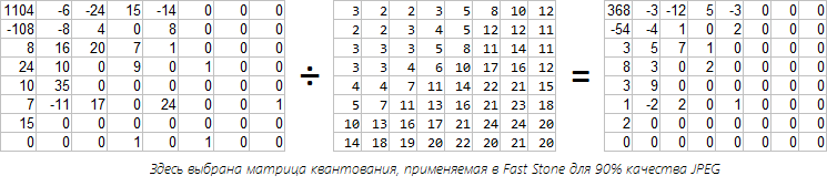
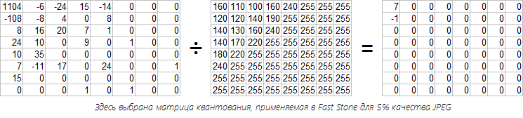
Two examples illustrate the process:

• One showing moderate compression (90% quality in FastStone)
• Another at 5% quality, reducing blocks to near-uniform colors

100% quality still produces minor artifacts due to rounding errors, though they are imperceptible to humans.

Encoding

This section develops Huffman coding concepts through progressive examples.

Example 0: Repetitive sequences can be abbreviated using symbol references.

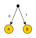
Example 1: Three symbols (A, B, C) require 2 bits each (6 bits total).

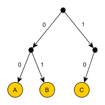
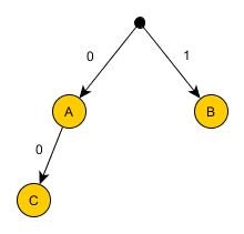
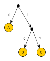
Example 2: Demonstrates the prefix-free code requirement — no code can begin with another code.

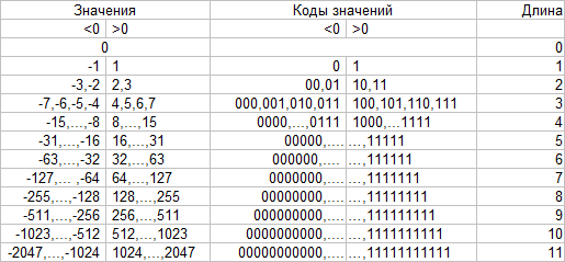
Example 3: The general case shows that optimal code lengths relate to symbol frequency through the formula s = -log₂p.

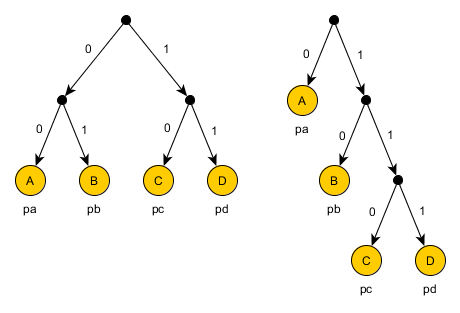
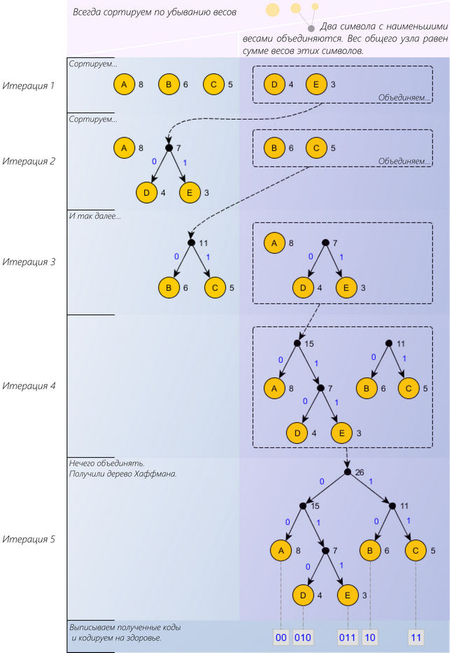
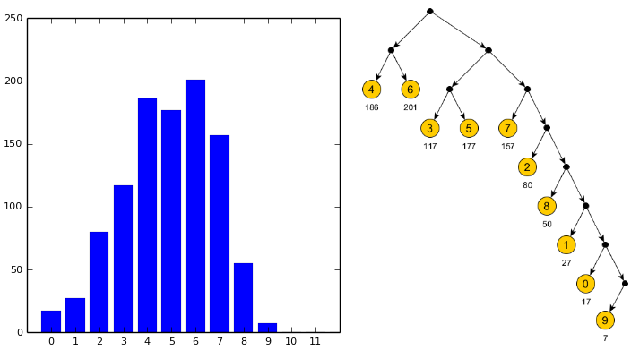
Example 4: The complete Huffman algorithm:

1. Sort symbols by frequency (descending)
2. Repeatedly combine the two lowest-weight symbols
3. Assign codes by tree traversal

The algorithm then applies to JPEG components:

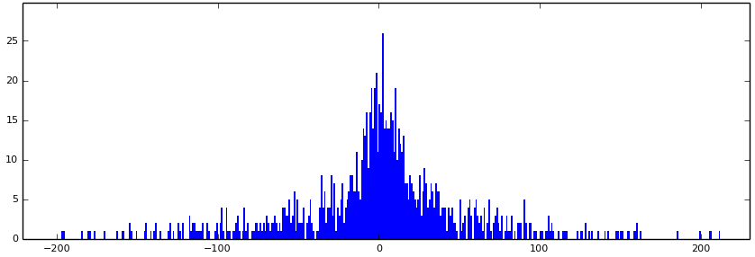
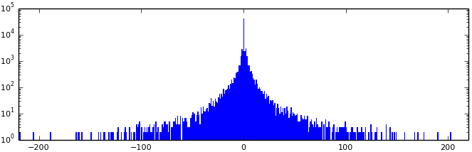
DC coefficients (average block values): Stored as differences between adjacent blocks, encoded with (Huffman length code, value) pairs.

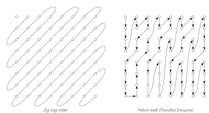
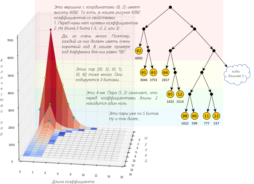
AC coefficients (remaining details): Uses "zig-zag" scan order to group zeros efficiently, then encodes pairs combining (zeros before non-zero value, coefficient length).

A critical JPEG detail: the pair (quantity of preceding zeros, AC length) creates an 8-bit value where codes are generated rather than stored directly. The special marker (0,0) indicates all remaining values are zero.

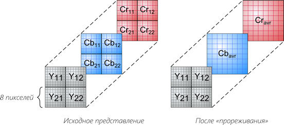
Color Images

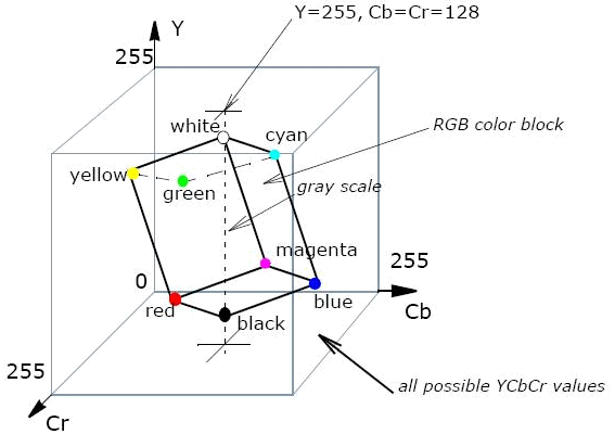
Rather than encoding RGB channels separately (tripling the work), JPEG uses the YCbCr color model, which separates:

• Y: Luminance (brightness)
• Cb, Cr: Chrominance (color differences)

Since human vision is more sensitive to brightness than color, the Cb and Cr channels are typically downsampled (reduced resolution) by factors like 2x2 or 4x2 blocks.

Common configurations:

• Grayscale (1 channel)
• YCbCr (3 channels)
• RGB (3 channels)
• CMYK (4 channels, problematic in some software)

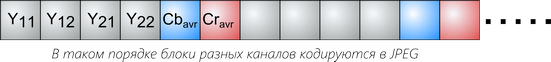
Each 8x8 block is encoded separately using the previously described DCT + Huffman process.

And a Few More Things

Progressive mode: DCT coefficients are decomposed into layers. The initial transmission provides DC values (8x8 pixel blocks), subsequent passes refine with rounded AC coefficients, creating gradual quality improvement during slow downloads.

Lossless mode: Eliminates DCT entirely. Predicts pixel values from three neighbors, encodes prediction errors using Huffman coding. Rarely used.

Hierarchical mode: Creates multi-resolution layer pyramids. The coarse layer is encoded normally, subsequent layers store differences via Haar wavelets. Uncommon.

Arithmetic coding: An alternative to Huffman offering approximately 10% better compression through fractional-bit encoding. Rarely supported due to patent restrictions.

Understanding JPEG's layered approach — vector representation, Fourier decomposition, quantization, and entropy coding — provides intuition applicable across signal processing domains. The compression principle always involves finding and describing patterns.