JPEG Decoding for Beginners
A step-by-step walkthrough of the JPEG decoding process using a real 16x16 pixel image, covering everything from reading file markers and Huffman tables to performing inverse DCT and color space conversion.
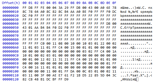
[FF D8]
If you want to understand how a JPG file works, grab a compiler and a hex editor — we're going to decode it step by step.
For this article, I used a heavily compressed Google favicon (16×16 pixels) as an example. The description is somewhat simplified but should be sufficient for understanding the specification.
[FF D8] — the start of image marker, always found at the very beginning of every JPG file.
The following bytes [FF FE] indicate the beginning of a comment section. The next 2 bytes [00 04] specify the section length. The values [3A 29] are the comment itself — the ASCII codes for ":" and ")", i.e., a smiley face emoticon visible in the right panel of the hex editor.
A Little Theory
Here's a brief overview of the key processes in JPEG compression:
- Color space conversion from RGB to YCbCr
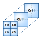
- Channel subsampling — reducing the Cb and Cr chrominance channels (e.g., 2:1 reduction both horizontally and vertically)
- Dividing the image into 8×8 blocks
- Discrete Cosine Transform (DCT) — applied to each 8×8 block, producing a matrix of 64 coefficients
- The top-left coefficient is the DC coefficient (the most important one), while the remaining 63 are AC coefficients
- Quantization — multiplying by the quantization matrix coefficients (this is where the lossy compression happens)
- Huffman encoding — lossless compression of the quantized coefficients
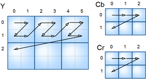
Data for blocks is interleaved in small portions: Y₀₀Y₁₀Y₀₁Y₁₁Cb₀₀Cr₀₀Y₂₀…
Reading the File
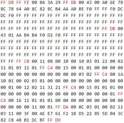
A JPEG file is structured as a sequence of segments, each preceded by a marker (2 bytes, where the first byte is always [FF]). Most segments also store their length in the following 2 bytes.

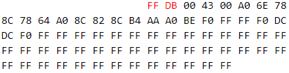
DQT Marker [FF DB] — Quantization Table
- [00 43] — Section length: 67 bytes
- [0_] — Value precision: 0 (0 = 1 byte, 1 = 2 bytes)
- [_0] — Table ID: 0
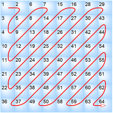
The remaining 64 bytes fill an 8×8 table in zigzag order:
Quantization matrix values (in hex):
[A0 6E 64 A0 F0 FF FF FF]
[78 78 8C BE FF FF FF FF]
[8C 82 A0 F0 FF FF FF FF]
[8C AA DC FF FF FF FF FF]
[B4 DC FF FF FF FF FF FF]
[F0 FF FF FF FF FF FF FF]
[FF FF FF FF FF FF FF FF]
[FF FF FF FF FF FF FF FF]
In decimal:
[160 110 100 160 240 255 255 255]
[120 120 140 190 255 255 255 255]
[140 130 160 240 255 255 255 255]
[140 170 220 255 255 255 255 255]
[180 220 255 255 255 255 255 255]
[240 255 255 255 255 255 255 255]
[255 255 255 255 255 255 255 255]
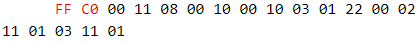
[255 255 255 255 255 255 255 255]SOF0 Marker [FF C0] — Baseline DCT
- [00 11] — Section length: 17 bytes
- [08] — Precision: 8 bits
- [00 10] — Image height: 16 pixels
- [00 10] — Image width: 16 pixels
- [03] — Number of channels: 3
Channel 1:
- [01] — Channel ID: 1 (Y)
- [2_] — Horizontal sampling factor (H₁): 2
- [_2] — Vertical sampling factor (V₁): 2
- [00] — Quantization table ID: 0
Channel 2:
- [02] — Channel ID: 2 (Cb)
- [1_] — Horizontal sampling factor (H₂): 1
- [_1] — Vertical sampling factor (V₂): 1
- [01] — Quantization table ID: 1
Channel 3:
- [03] — Channel ID: 3 (Cr)
- [1_] — Horizontal sampling factor (H₃): 1
- [_1] — Vertical sampling factor (V₃): 1
- [01] — Quantization table ID: 1
Hmax = 2, Vmax = 2. Channel i is subsampled by a factor of Hmax/Hi horizontally and Vmax/Vi vertically.
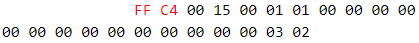
DHT Marker [FF C4] — Huffman Table
Number of codes per length:
Length:       1  2  3  4  5  6  7  8  9 10 11 12 13 14 15 16
Code count: [01 01 00 00 00 00 00 00 00 00 00 00 00 00 00 00]
Values: [03] and [02]. This means there are 2 codes total: one of length 1 with value 3, and one of length 2 with value 2.
The Huffman tree is built as follows:
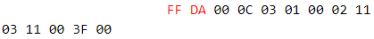
SOS Marker [FF DA] — Start of Scan
- [00 0C] — Section length: 12 bytes
- [03] — Number of channels: 3
Channel 1 (Y):
- [01] — Channel ID: 1
- [0_] — DC Huffman table: 0
- [_0] — AC Huffman table: 0
Channel 2 (Cb):
- [02] — Channel ID: 2
- [1_] — DC Huffman table: 1
- [_1] — AC Huffman table: 1
Channel 3 (Cr):
- [03] — Channel ID: 3
- [1_] — DC Huffman table: 1
- [_1] — AC Huffman table: 1
[00], [3F], [00] — parameters for progressive mode (not covered in this article).
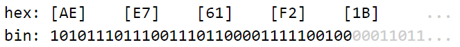
Encoded Data
After the SOS marker, the actual encoded image data begins.
Finding the DC Coefficient
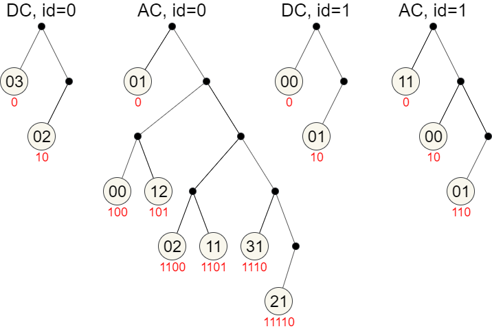
- Read the bit sequence (if you encounter [FF 00], treat it as [FF] — it's not a marker). Traverse the Huffman tree following the bits: 0 means go left, 1 means go right. Stop when you reach a leaf node.
- Extract the node's value. A value of 0 means the coefficient is 0. Otherwise, the value tells you how many subsequent bits represent the coefficient.
- If the first bit is 1, keep the value as-is. Otherwise, compute: DC = value − 2length + 1. Place the result in the zigzag's top-left position.
Finding AC Coefficients
- Continue reading the bit sequence.
- Get the node's value. A value of 0 means fill the remaining positions in the matrix with zeros. Otherwise, the high nibble tells you how many zeros precede the coefficient, and the low nibble tells you the bit length of the coefficient.
- Apply the same sign conversion logic as for DC coefficients.
Continue until the entire 8×8 matrix is filled or a zero code (end of block) is encountered.
Result — the first Y-channel coefficient matrix (before dequantization):
[ 2  0  3  0  0  0  0  0]
[ 0  1  2  0  0  0  0  0]
[ 0 -1 -1  0  0  0  0  0]
[ 1  0  0  0  0  0  0  0]
[ 0  0  0  0  0  0  0  0]
[ 0  0  0  0  0  0  0  0]
[ 0  0  0  0  0  0  0  0]
[ 0  0  0  0  0  0  0  0]
The remaining three Y-channel matrices (decoded the same way):
[-4  1  1  1  0  0  0  0]    [ 5 -1  1  0  0  0  0  0]    [-4  2  2  1  0  0  0  0]
[ 0  0  1  0  0  0  0  0]    [-1 -2 -1  0  0  0  0  0]    [-1  0 -1  0  0  0  0  0]
[ 0 -1  0  0  0  0  0  0]    [ 0 -1  0  0  0  0  0  0]    [-1 -1  0  0  0  0  0  0]
[ 0  0  0  0  0  0  0  0]    [-1  0  0  0  0  0  0  0]    [ 0  0  0  0  0  0  0  0]
[ 0  0  0  0  0  0  0  0]    [ 0  0  0  0  0  0  0  0]    [ 0  0  0  0  0  0  0  0]
[ 0  0  0  0  0  0  0  0]    [ 0  0  0  0  0  0  0  0]    [ 0  0  0  0  0  0  0  0]
[ 0  0  0  0  0  0  0  0]    [ 0  0  0  0  0  0  0  0]    [ 0  0  0  0  0  0  0  0]
[ 0  0  0  0  0  0  0  0]    [ 0  0  0  0  0  0  0  0]    [ 0  0  0  0  0  0  0  0]
Note that DC coefficients are stored as differences from the previous DC coefficient of the same channel:
- Matrix 2 DC: 2 + (−4) = −2
- Matrix 3 DC: −2 + 5 = 3
- Matrix 4 DC: 3 + (−4) = −1
Corrected matrices (with absolute DC values):
[-2  1  1  1  0  0  0  0]    [ 3 -1  1  0  0  0  0  0]    [-1  2  2  1  0  0  0  0]
[ 0  0  1  0  0  0  0  0]    [-1 -2 -1  0  0  0  0  0]    [-1  0 -1  0  0  0  0  0]
[ 0 -1  0  0  0  0  0  0]    [ 0 -1  0  0  0  0  0  0]    [-1 -1  0  0  0  0  0  0]
[ 0  0  0  0  0  0  0  0]    [-1  0  0  0  0  0  0  0]    [ 0  0  0  0  0  0  0  0]
[ 0  0  0  0  0  0  0  0]    [ 0  0  0  0  0  0  0  0]    [ 0  0  0  0  0  0  0  0]
[ 0  0  0  0  0  0  0  0]    [ 0  0  0  0  0  0  0  0]    [ 0  0  0  0  0  0  0  0]
[ 0  0  0  0  0  0  0  0]    [ 0  0  0  0  0  0  0  0]    [ 0  0  0  0  0  0  0  0]
[ 0  0  0  0  0  0  0  0]    [ 0  0  0  0  0  0  0  0]    [ 0  0  0  0  0  0  0  0]
The Cb and Cr channel matrices:
Cb:                           Cr:
[-1  0  0  0  0  0  0  0]    [ 0  0  0  0  0  0  0  0]
[ 1  1  0  0  0  0  0  0]    [ 1 -1  0  0  0  0  0  0]
[ 0  0  0  0  0  0  0  0]    [ 1  0  0  0  0  0  0  0]
[ 0  0  0  0  0  0  0  0]    [ 0  0  0  0  0  0  0  0]
[ 0  0  0  0  0  0  0  0]    [ 0  0  0  0  0  0  0  0]
[ 0  0  0  0  0  0  0  0]    [ 0  0  0  0  0  0  0  0]
[ 0  0  0  0  0  0  0  0]    [ 0  0  0  0  0  0  0  0]
[ 0  0  0  0  0  0  0  0]    [ 0  0  0  0  0  0  0  0]
Calculations
Dequantization
We multiply each coefficient matrix element by the corresponding element of the quantization table.

Y-channel matrices after dequantization:
[ 320    0  300  0  0  0  0  0]    [-320  110  100  160  0  0  0  0]
[   0  120  280  0  0  0  0  0]    [   0    0  140    0  0  0  0  0]
[   0 -130 -160  0  0  0  0  0]    [   0 -130    0    0  0  0  0  0]
[ 140    0    0  0  0  0  0  0]    [   0    0    0    0  0  0  0  0]
[   0    0    0  0  0  0  0  0]    [   0    0    0    0  0  0  0  0]
[   0    0    0  0  0  0  0  0]    [   0    0    0    0  0  0  0  0]
[   0    0    0  0  0  0  0  0]    [   0    0    0    0  0  0  0  0]
[   0    0    0  0  0  0  0  0]    [   0    0    0    0  0  0  0  0]

[ 480 -110  100  0  0  0  0  0]    [-160  220  200  160  0  0  0  0]
[-120 -240 -140  0  0  0  0  0]    [-120    0 -140    0  0  0  0  0]
[   0 -130    0  0  0  0  0  0]    [-140 -130    0    0  0  0  0  0]
[-140    0    0  0  0  0  0  0]    [   0    0    0    0  0  0  0  0]
[   0    0    0  0  0  0  0  0]    [   0    0    0    0  0  0  0  0]
[   0    0    0  0  0  0  0  0]    [   0    0    0    0  0  0  0  0]
[   0    0    0  0  0  0  0  0]    [   0    0    0    0  0  0  0  0]
[   0    0    0  0  0  0  0  0]    [   0    0    0    0  0  0  0  0]
Cb and Cr matrices after dequantization:
Cb: Cr:
[-170 0 0 0 0 0 0 0] [ 0 0 0 0 0 0 0 0]
[ 180 210 0 0 0 0 0 0] [ 180 -210 0 0 0 0 0 0]
[ 0 0 0 0 0 0 0 0] [ 240 0 0 0 0 0 0 0]
[ 0 0 0 0 0 0 0 0] [ 0 0 0 0 0 0 0 0]
[ 0 0 0 0 0 0 0 0] [ 0 0 0 0 0 0 0 0]
[ 0 0 0 0 0 0 0 0] [ 0 0 0 0 0 0 0 0]
[ 0 0 0 0 0 0 0 0] [ 0 0 0 0 0 0 0 0]
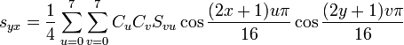
[ 0 0 0 0 0 0 0 0] [ 0 0 0 0 0 0 0 0]Inverse DCT

The formula for the inverse DCT:
syx = (1/4) × Σu=0..7 Σv=0..7 CuCv × Svu × cos((2x+1)uπ/16) × cos((2y+1)vπ/16)
where Cx = 1/√2 when x = 0, and Cx = 1 otherwise.
After computing the inverse DCT and rounding, the first Y-channel block gives:
[138  92  27 -17 -17  28  93 139]
[136  82   5 -51 -55  -8  61 111]
[143  80  -9 -77 -89 -41  32  86]
[157  95   6 -62 -76 -33  36  86]
[147 103  37 -12 -21  11  62 100]
[ 87  72  50  36  37  55  79  95]
[-10   5  31  56  71  73  68  62]
[-87 -50   6  56  79  72  48  29]
After adding 128 and clamping values to the [0, 255] range:

The Cb and Cr matrices after inverse DCT (these are 8×8 because Cb/Cr are not subsampled into multiple blocks):
Cb:                                         Cr:
[ 60  52  38  20   0 -18 -32 -40]    [ 19  27  41  60  80  99 113 120]
[ 48  41  29  13  -3 -19 -31 -37]    [  0   6  18  34  51  66  78  85]
[ 25  20  12   2  -9 -19 -27 -32]    [-27 -22 -14  -4   7  17  25  30]
[ -4  -6  -9 -13 -17 -20 -23 -25]    [-43 -41 -38 -34 -30 -27 -24 -22]
[-37 -35 -33 -29 -25 -21 -18 -17]    [-35 -36 -39 -43 -47 -51 -53 -55]
[-67 -63 -55 -44 -33 -22 -14 -10]    [ -5  -9 -17 -28 -39 -50 -58 -62]
[-90 -84 -71 -56 -39 -23 -11  -4]    [ 32  26  14  -1 -18 -34 -46 -53]
[-102 -95 -81 -62 -42 -23  -9  -1]    [ 58  50  36  18  -2 -20 -34 -42]
Values are then clamped to [0, 255] after adding 128.
YCbCr to RGB Conversion

Since the Cb and Cr channels were subsampled (each 8×8 Cb/Cr block covers the entire 16×16 image), we need to upsample them to match the Y channel's resolution. Each Cb/Cr pixel maps to a 2×2 block of Y pixels.
The conversion formulas:
- R = round(Y + 1.402 × (Cr − 128))
- G = round(Y − 0.34414 × (Cb − 128) − 0.71414 × (Cr − 128))
- B = round(Y + 1.772 × (Cb − 128))
Final RGB values for the upper-left 8×8 block:
R channel:
[255 249 195 149 169 215 255 255]
[255 238 172 116 131 179 255 255]
[255 209 127  58  64 112 209 255]
[255 224 143  73  76 120 212 255]
[217 193 134  84  86 118 185 223]
[177 162 147 132 145 162 201 218]
[ 57  74 101 125 144 146 147 142]
[  0  18  76 125 153 146 128 108]
G channel:
[220 186 118  72  67 113 172 205]
[220 175  95  39  29  77 139 190]
[238 192 100  31  16  64 132 185]
[238 207 116  46  28  72 135 186]
[255 242 175 125 113 145 193 231]
[226 211 188 173 172 189 209 226]
[149 166 192 216 230 232 225 220]
[ 73 110 167 216 239 232 206 186]
B channel:
[255 255 250 204 179 225 255 255]
[255 255 227 171 141 189 224 255]
[255 255 193 124  90 138 186 239]
[255 255 209 139 102 146 189 240]
[255 255 203 153 130 162 195 233]
[255 244 216 201 189 206 211 228]
[108 125 148 172 183 185 173 168]
[ 32  69 123 172 192 185 154 134]
Conclusion
I am not a specialist in this field, but I enjoy figuring out how things work. When I decided to understand the JPEG format, I searched for a worked example with real numbers but couldn't find one — only theoretical descriptions and convoluted specifications. So I did the decoding myself and tried to document it as clearly as possible. I hope this article saves someone some time.
Here are some resources I found helpful:
- ru.wikipedia.org/JPEG — a good introductory overview
- en.wikipedia.org/JPEG — more detail on the encoding/decoding process
- JPEG Standard (ISO/IEC 10918-1 ITU-T Recommendation T.81) — the official specification
- impulseadventure.com/photo — great articles with Huffman tree construction examples
- JPEGsnoop — a utility for extracting detailed information from JPEG files
[FF D9]