Radars and How to Hide From Them. Part 1: Basics of Radar

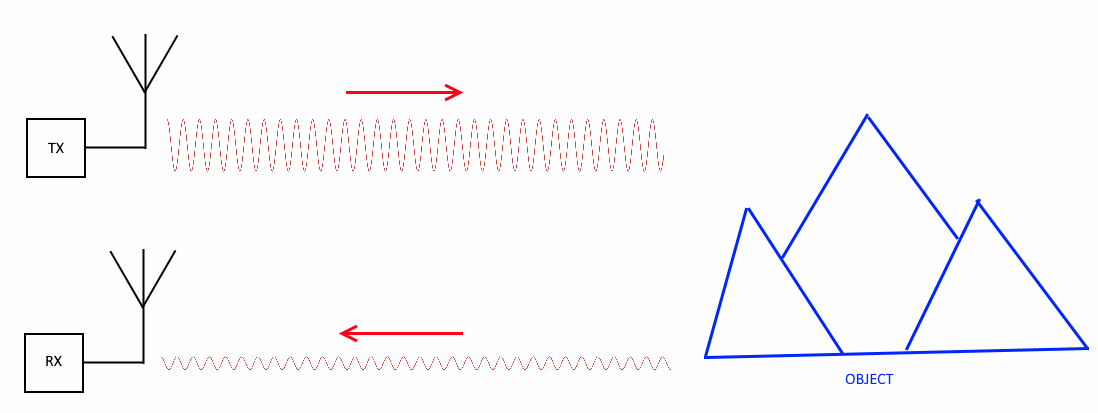
A radar is, by definition, a RAdio Detection And Ranging device — an instrument for detecting the presence of a target and measuring the distance to it using radio waves. In its simplest form a radar is not very different from ordinary radio. We set up a radio transmitter, set up a radio receiver, point both antennas toward the "target" and listen. If an object that reflects radio waves is present in the direction the waves are travelling, a portion of those waves will bounce back and we will pick up the transmitter's signal at the receiver. If there is no object — we hear nothing.

Because of its simplicity, this scheme often emerged spontaneously when engineers were merely trying to establish radio communications, so the effect was discovered almost as soon as radio found practical use. The idea was obvious enough that as early as 1904 the German inventor Christian Hülsmeyer demonstrated the first working radar prototype capable of detecting ships in fog at distances up to 3 km. A radar of this kind resembles a searchlight that we sweep through the darkness hoping to catch a distant glint. It cannot measure range, but by rotating the receiver's antenna one can find the direction in which the signal is strongest and thus locate a target's bearing. This is precisely the principle behind the vast majority of radio-homing guidance systems on anti-aircraft missiles. The system's simplicity reduces the size and cost of the seeker head, and the inability to measure range is irrelevant there. An especially simple and cheap variant places only a receiver on the missile ("semi-active homing") while the transmitter stays on the ground launcher or launching aircraft. This is the so-called bistatic configuration, where transmitter and receiver are separated by a significant distance, as opposed to the more familiar monostatic configurations that combine transmitter and receiver into a single unit.

Antenna Beam Width

Here we immediately hit the first problem. Radio waves are quite difficult to shape into a narrow beam. For an antenna of width d operating at wavelength λ, the beam width in radians in the ideal case is θ = 2λ/(πd). In practice the beam is wider; for a parabolic dish — which offers excellent directivity — it works out to roughly θ = 1.2 λ/d, or in the more convenient unit of degrees: θ = 70° × λ/d.

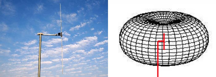
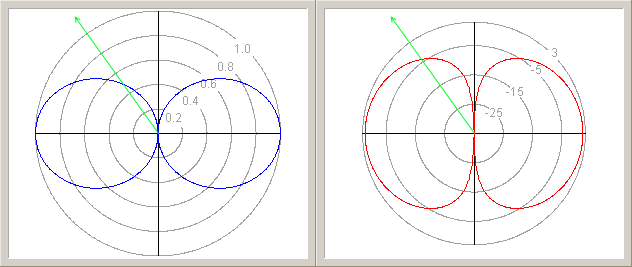
Early radio transmitters operated around 1 MHz, giving λ ≈ 300 m, making any useful directivity essentially impossible. Even the "shortwave" transmitters that appeared in the 1920s had λ = 10–100 m, which demanded antenna dimensions of tens of metres. Engineers had to be clever. To understand what they came up with, we need the concept of the antenna radiation pattern — a graph showing how strongly an antenna radiates (or receives) in a given direction. For a dipole antenna consisting of two vertical conductors of equal size, the full 3-D pattern looks like a torus (doughnut) with the conductors running through its centre.

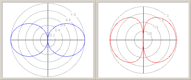
Working in 3-D is inconvenient, so in practice the pattern is examined in cross-section. For a half-wave dipole (size λ/2) that cross-section looks like the figure below. The blue curve is plotted on a linear scale; the red one on a logarithmic scale. Using it is straightforward: to find the antenna gain in the direction shown by the green arrow, find the intersection of the green line with the blue or red curve. In linear units the gain is roughly 0.5; in logarithmic units roughly −3 dB.

Decibels and Logarithmic Scale

Radio engineering almost always uses logarithmic units, because virtually every factor affecting a signal is multiplicative: the output Y is derived from input X as Y = A · X for some factor A (such as antenna gain). When you take logarithms, multiplications become additions — log(Y) = log(A) + log(X) — and adding numbers is far easier than multiplying them. The base-10 logarithm gives the unit called the bel. A gain of 1 bel equals a factor of 10: 1 bel = log₁₀(10). Since 1 bel is rather large, in practice the decibel (dB), one-tenth of a bel, is used — a gain factor of √10 ≈ 1.259. Positive numbers represent amplification; negative numbers represent attenuation. For example, the −3 dB mentioned above equals a factor of 10^(−3/10) = 1/∛(10³) ≈ 0.5.

The logarithmic scale not only gives values in convenient decibels but also reveals subtle details. For instance, the radiation pattern of a parabolic dish plotted on a logarithmic scale clearly shows that the antenna radiates (and receives) a small but non-negligible portion of its signal from the sides — the so-called sidelobe pattern. As we will soon see, this is extremely important in radar.

Finding the Minimum: Null Seeking and Loop Antennas

Recalling what we said earlier: to get a nicely directional pattern like the parabolic dish, the antenna must be many times larger than the wavelength λ. A practical "dish" would need to be about a kilometre across — clearly impossible. With antennas that engineers could actually build, the radiation pattern was, shall we say, not very directional.

The first "hack" inventors hit upon was searching not for a signal maximum but for its minimum — the so-called null. Looking at the pattern above, the region where the signal goes to zero is clearly much narrower, and therefore can be located more precisely. The second hack was the use of loop antennas, which produce quite a sharp null even when their size is only λ/10.

Such a system was already usable: compact, yet capable of finding the bearing to a signal source with an error of only 1–2 degrees. In practice, however, it was awkward: when the antenna pointed directly at the source, its signal disappeared — indistinguishable from there being no signal at all. And was a weak signal weak because you were pointing correctly, or because the source was far away? Moreover, the two nulls made direction ambiguous. Engineers later solved this by combining a loop with a dipole to produce the so-called cardioid antenna.

The Cardioid Antenna and the Radio Compass

The cardioid antenna exploits the fact that a dipole and a loop receive signals with a different delay (phase): the dipole responds to the electric component of the electromagnetic wave while the loop responds to the magnetic component, which is shifted 90° in phase. A wave arriving from the "front" produces a +90° delay; one from the "back" produces −90°. Using a phase shifter we can add another 90°, so the front-arriving wave has a total shift of 180° and the rear-arriving wave has 0°. If you remember how a sine wave works, you will see that in the first case the signals from the loop and dipole cancel, while in the second they reinforce. By choosing the system parameters carefully, the cancellation from the front can be made nearly complete while the signal from the rear is strengthened.

In practice the phase shifter is switchable between +90° and −90°, reversing the direction of the null. Switching is often done automatically at an audible frequency (e.g. 300 Hz). When the antenna points at the source, the output jumps between "high" and "low" at 300 Hz — heard as a loud tone. When it does not, the swing collapses and the tone disappears, while at all times the presence of a signal is confirmed. This scheme appeared in the 1930s and survives to this day as the radio compass, which was the foundation of air navigation until GPS became widespread.

The Inverse Fourth-Power Law

Now let us return to radars proper. The second problem facing their inventors was insufficient received power. Any electromagnetic wave has a small focal region where its beam diameter is at a minimum; beyond roughly ten wavelengths from that focus the beam diameter grows in proportion to distance. For a continuous beam of uniform power, the energy is spread across an area proportional to d² at distance d from the focal point, so energy density falls as 1/d². In practical antennas the focal point is essentially the antenna itself, so d is always the distance to the antenna.

Now for the calculation. We launch electromagnetic waves at power W₀ toward an object at distance d₁ from the transmitter antenna and d₂ from the receiver antenna. Assuming W₀ is radiated equally in all directions, the power density near the object is W₁ = W₀/(4πd₁²). Real antennas concentrate energy in a preferred direction; the ratio of the energy actually delivered to the object versus what an isotropic radiator would deliver is called the transmitter antenna gain G₁:

W₁ = G₁W₀/(4πd₁²)

If the object's projected area toward the incoming wave is S₁, it intercepts power W₂ = W₁S₁. Assuming this is re-radiated equally in all directions, the power per unit area at distance d₂ is W₃ = W₂/(4πd₂²). In practice neither uniform re-radiation nor perpendicular objects exist, so S₁ is replaced by a computed quantity called the radar cross-section (RCS). Sometimes it is described as the area of a metal plate that would return the same signal power, but this description is only approximately true because RCS depends heavily on shape and even on wavelength. More precisely, RCS is simply a coefficient in the formula.

Letting S₂ denote the effective aperture of the receiving antenna, the received power is:

W₄ = W₀ · G₁/(4πd₁²) · S₁/(4πd₂²) · S₂

For a monostatic system (d₁ ≈ d₂ ≈ d) this simplifies to:

W₄ = W₀ · G₁ · S₁ · S₂ / ((4π)² · d⁴)

The key result: W₄ ∝ W₀/d⁴. Received signal power falls with the fourth power of distance. Doubling the range reduces the signal by a factor of 16. Building a practical radar therefore required either a very powerful transmitter, a large receiving antenna, or a highly directional transmitting antenna — or all three — to overcome this effect. The need for range was most acute in air-defence radars: an air target covers 20–25 km in about three minutes, barely enough time to aim guns and nowhere near enough to scramble fighters needing up to ten minutes to reach altitude. Early long-range systems therefore used antennas hundreds of metres across.

Chain Home and the Bellini-Tosi Goniometer

The world's first operational early-warning radar, Chain Home (1937), capable of detecting aircraft at up to 200 km, used an antenna system roughly 200 × 100 metres supported by several tall towers.

This was expensive in itself, but it also posed a severe practical question: how do you rotate such a structure to determine bearings? The answer was the radio goniometer, invented in 1909 by Italians Ettore Bellini and Alessandro Tosi. They realised that the signal received on a large fixed antenna could be reproduced at a small scale inside a special chamber. By rotating a small "goniometer" antenna inside that "scale model of the real world" they achieved the same effect as rotating the full-sized structure. The Bellini-Tosi system used two loop antennas; in 1919 Briton Frank Adcock invented a similar scheme for four dipole antennas that reduced pick-up of unwanted signals. Vertically polarised signals detected this way reflect poorly from the ionosphere and the ground. Goniometers allowed the massive radar antenna to remain stationary while only a small component inside the receiver rotated — a conceptual forerunner of the phased-array antennas we will meet later.

For a while the investment in such complex and expensive systems (instead of, say, building more aircraft) seemed questionable, but the first combat use of radar in the Battle of Britain settled the matter. Attackers normally held a large advantage: they could concentrate all their aircraft at one point while defenders had to spread out to protect many targets, and targets were often bombed before a response could be organised. Thanks to radar, the British were able to concentrate their counter-strikes and meet the Germans before they reached the coast. The absence of radar proved a decisive and fatal weakness for the Italians at Cape Matapan and for the Japanese at Midway. The years of World War II became a period of extraordinarily rapid radar development.

The SCR-270 and the Move to Shorter Wavelengths

A 100 × 200 metre antenna was not what the military wanted. As the formula above shows, the required antenna size could be greatly reduced by shortening the wavelength λ. The American SCR-270 radar operating at 200 MHz needed an antenna an order of magnitude smaller than Chain Home (which operated at 20 MHz) for equal or better range, required no goniometer, and could be transported relatively easily.

Today frequencies below 40 MHz are used only by specialised over-the-horizon radars; even 200 MHz is considered quite "long-wave" and impractical. But pushing to shorter wavelengths ran into a sustained dead end for a long time: higher frequencies increased losses in transmitters and receivers, and "microwave" radiation with λ ≈ 10 cm and below was an entirely new world requiring completely different design approaches. Two devices broke that impasse.

The Klystron and the Magnetron

The klystron (USA) is a microwave amplifier. It was the first efficient solution in that field and — after many improvements — it remains so today. All the most powerful radio transmitters still use klystrons; modern semiconductor amplifiers cannot deliver a hundredth of the power of a large klystron, and large phased arrays with many amplifiers cost far more. The Americans failed to classify their invention, so it was widely used by both sides — including Germany.

The magnetron (Britain) was more specialised: it could only generate microwave radiation, and of rather low quality at that. But it produced truly enormous power in a very compact package and achieved conversion efficiencies up to 80%. Those qualities are why magnetrons are found today in every household microwave oven, where their weaknesses are irrelevant and their advantages obvious. Unlike with the klystron, the British classified this invention (sharing it only with the Allies after the war began), and it played a significant role in Allied technical superiority over Germany.

Compact, powerful microwave sources with λ ≈ 10–30 cm allowed WWII-era radars to shrink to the point where they could fit in fairly large aircraft. By the 1960s radar had moved to the "centimetric" band (λ ≈ 1–10 cm), which remains the primary radar band today. By the 1970s millimetre-wave radars had appeared, but here radar engineering ran seriously into atmospheric transparency limitations for the first time.

Frequency Bands and Atmospheric Absorption

Atmospheric absorption attenuates a signal by a factor of 10^(−0.1kd) over distance d (km), where k is the absorption coefficient in dB/km. For wavelengths above 1 cm (below 30 GHz), k does not exceed 0.01 dB/km, meaning even at 300 km the atmosphere attenuates the signal by no more than a factor of two. But above 70 GHz (λ < 4 mm), k exceeds 0.1 dB/km — a tenfold signal loss every 100 km. Millimetre-wave radars have therefore become a niche product used either at short ranges or in space. Sub-millimetre (terahertz) radars suffer attenuation above 1 dB/km and are limited to extremely short ranges — mainly body scanners in airport security.

Rain is another bane of short-wave radars. Even a light shower produces crippling absorption above 1 dB/km at frequencies above 20 GHz. Radars capable of operating through heavy rain must use frequencies below 5 GHz (λ > 6 cm).

These constraints led to the following primary radar frequency bands, each representing an optimal compromise between antenna size and atmospheric absorption:

• L-band (1–2 GHz, λ = 15–30 cm) — civil aviation radars
• S-band (2–4 GHz, λ = 7.5–15 cm) — maritime radars, weather radars, civil aviation radars, many long-range military radars
• C-band (3.6–8 GHz, λ = 4–8 cm) — radar altimeters
• X-band (8–12 GHz, λ = 25–40 mm) — one of the most widely used military and civil radar bands
• Ku-band (12–18 GHz, λ = 15–25 mm) — compact short-range radars, including familiar police speed guns

Continuous Wave Radar and the Doppler Effect

Having established the frequency band and the reasons it was chosen, let us return to how a radar works. So far we have examined the simplest scheme — continuous transmission — which only indicates whether an object is present in a given direction. That is sufficient for missile homing, and it also underlies some modern motion detectors, but we most commonly encounter it in police speed radars.

A signal reflected from a moving object changes its frequency slightly — a phenomenon known as the Doppler effect. A wave reflected in the direction of motion is compressed (higher frequency); one reflected away from the motion is stretched (lower frequency).

By measuring the frequency shift one can determine the object's velocity. This can be done with a comparatively simple circuit known as a frequency mixer. A mixer receiving signals at frequencies f₁ and f₂ produces outputs at f₁ + f₂ and |f₁ − f₂|. In the radar context, feeding the transmitted and received signals into the mixer yields a difference-frequency component that encodes the Doppler shift. For an ideal mixer this is the only low-frequency component in the output and can be isolated easily with a low-pass filter.

FMCW Radar: Measuring Range

The Doppler scheme can be reworked to measure distance rather than velocity by continuously varying the transmitted frequency. The reflected signal returns with a time delay corresponding to the target's range; during that delay the transmitted frequency has changed. Measuring the frequency difference between the current transmission and the received signal gives the delay, and from the delay we compute the range. This is the frequency-modulated continuous wave (FMCW) radar.

In the simplest variant the transmitted frequency varies in a sawtooth pattern — rising linearly to a maximum, then resetting to the start. The frequency difference maps directly to range for a stationary target. More sophisticated modulation schemes eliminate the ambiguous "reset" region and can additionally extract the Doppler component due to target motion. The result is an inexpensive, practical radar widely used today for short-range distance measurement.

The series continues in Part 2, Part 3, and Part 4.