Restoring Defocused and Motion-Blurred Images: A Practical Guide

In my previous article I described the theory behind restoring blurred and defocused images. That article generated a lot of interest, and it's time to move on to practice. I must say right away: the practice has turned out to be more interesting and extensive than I expected. There have been many discoveries, some of which I haven't seen described anywhere else.

At the end of the article, there's a link to a demo application with which you can experiment on your own images.

Let's Recall the Theory

The degradation of an image by an optical system (or motion) can be described by the convolution operation, where each pixel of the original image is "smeared" according to a certain pattern — the Point Spread Function (PSF). The PSF essentially shows what a single luminous point turns into after being distorted.

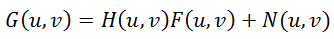
One of the most important properties of the Fourier transform comes to our rescue: convolution in the spatial domain is equivalent to simple multiplication in the frequency domain. That is:

G(u,v) = H(u,v) * F(u,v) + N(u,v)

where G is the Fourier transform of the distorted image, H is the Fourier transform of the PSF (also called the Optical Transfer Function — OTF), F is the Fourier transform of the original image, and N is noise.

The most obvious restoration method — simply dividing G by H — doesn't work in practice because noise gets amplified enormously at frequencies where H is close to zero.

The Wiener filter solves this problem by minimizing the mean-square error between the restored and original images:

F'(u,v) = [H*(u,v) / (|H(u,v)|² + K)] * G(u,v)

where H* is the complex conjugate of H, and K is a parameter related to the noise-to-signal ratio. In practice, K is selected manually — increasing it reduces noise but also reduces sharpness, while decreasing it increases sharpness but amplifies noise artifacts.

Methods of Obtaining the PSF

The PSF is what we need to know (or estimate) to restore the image. There are several ways to obtain it:

1. Modeling of optical systems. If we know the exact characteristics of the lens, we can simulate its PSF. In practice, this is almost impossible for multi-element lenses with complex aberrations.
2. Direct observation. We photograph a point light source through the same optical system with the same defocus. This gives us the PSF directly.
3. Indirect computation. If we have both the original sharp image and the blurred version, dividing their Fourier transforms gives us the OTF, and hence the PSF.

About Bokeh

Before we proceed, it's worth discussing bokeh — the quality of the out-of-focus blur produced by a lens. Bokeh is directly related to the PSF shape.

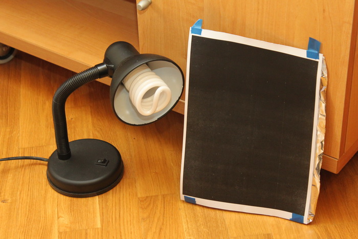
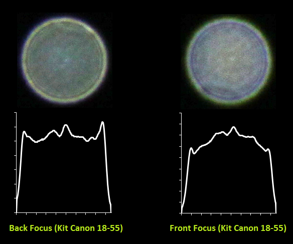
For simple lenses, the PSF of defocus is a filled circle (called the circle of confusion). But real lenses produce more complex patterns:

• Neutral bokeh — the PSF is close to a uniform filled circle
• Soft bokeh — the edges of the circle are dimmer than the center (often considered more pleasing)
• Harsh bokeh — the edges are brighter than the center (ring-shaped PSF, often considered less pleasing)

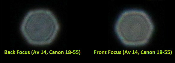
The type of bokeh — soft or harsh — also depends on whether the subject is in front of or behind the focal plane. With front focus, the bokeh tends to be softer, and with back focus, it tends to be harsher (or vice versa, depending on the lens design).

Additionally, at the edges of the frame, the PSF becomes elliptical rather than circular due to vignetting and the angle of incident light. This means the blur at the center of the frame and at the edges has a different character — an important consideration for deconvolution.

PSF — Direct Observation

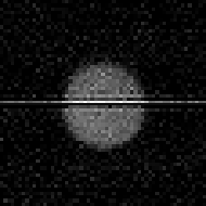
The most reliable way to obtain the PSF is to photograph an actual point light source. I constructed a simple apparatus: a 200-watt lamp behind a sheet of black paper backed with aluminum foil, with a tiny pinhole punched through. This creates a bright point source of light.

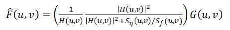
I photographed this point source with several Canon lenses at different aperture values and defocus amounts. The results were quite revealing:

You can clearly see the differences between lenses: some produce nearly perfect circles (neutral bokeh), while others show pronounced rings (harsh bokeh). Chromatic aberrations are also visible — the PSF is slightly different for red, green, and blue channels, which contributes to color fringing in out-of-focus areas.

For deconvolution, we can use either the full-color PSF or convert it to grayscale. Using the grayscale version is simpler and works well enough in most cases.

PSF — Computation or Indirect Observation

If we have a sharp reference image and its blurred version (photographed with the same defocus), we can compute the PSF. By dividing the Fourier transform of the blurred image by the Fourier transform of the sharp image, we obtain the OTF:

H(u,v) = G(u,v) / F(u,v)

Then an inverse Fourier transform gives us the PSF. In practice, this division is noisy, and the resulting PSF needs to be cleaned up — typically by thresholding and smoothing.

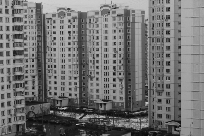
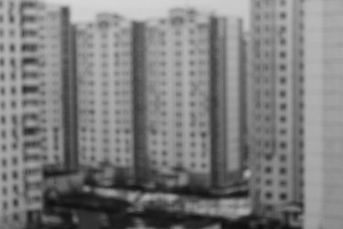
I tested this method by photographing a printed test pattern with controlled defocus. The computed PSF matched the directly observed PSF very closely, confirming the validity of this approach.

Edge Effects

One of the most unpleasant artifacts in deconvolution is "ringing" — oscillating patterns that appear at sharp boundaries in the image. This is a fundamental consequence of the Fourier transform: it assumes the image is periodic (repeats infinitely), so any discontinuity at the image borders creates artificial high-frequency content.

My solution is to preprocess the image before deconvolution:

1. Create a blurred copy of the input image (using a large Gaussian blur)
2. Create a weight mask that transitions smoothly from 0 at the edges to 1 in the center
3. Blend the original and blurred images using this mask: at the edges, we use the blurred version (which wraps smoothly), and in the center, we use the original

This effectively eliminates ringing artifacts at image boundaries while preserving detail in the center of the image.

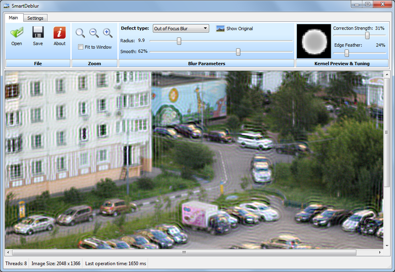
Practical Implementation

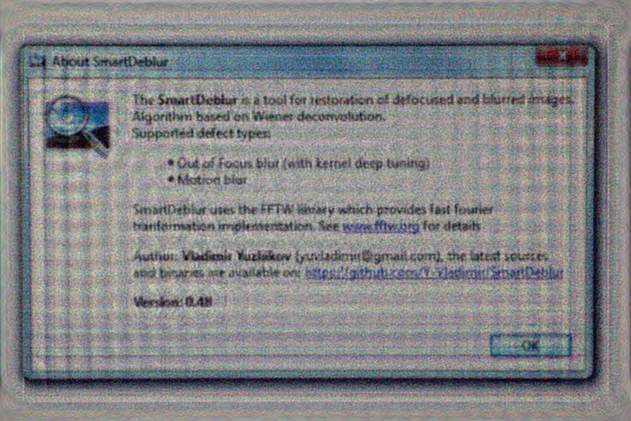
I've created a demo application called SmartDeblur, written in C++ using the Qt framework and the FFTW library for fast Fourier transforms.

Key features:

• Processing an image of 2048x1500 pixels takes approximately 300 ms in preview mode (quarter resolution) and about 1.5 seconds at full resolution
• Supports both defocus blur (circular PSF) and motion blur (linear PSF)
• Real-time parameter adjustment
• The application surpasses commercial analogs in speed by tens of times

The application and source code are available on GitHub under the GPL v3 license.

Comparison with Commercial Software

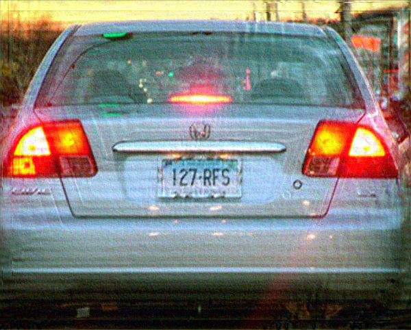
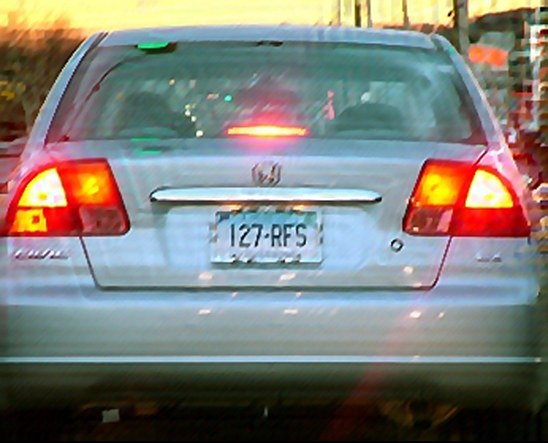
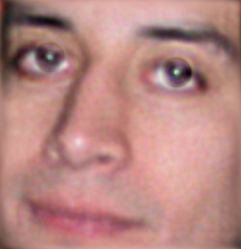
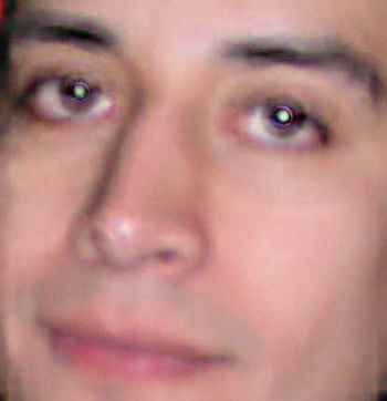
I compared SmartDeblur's results with two popular commercial solutions: Topaz InFocus and Focus Magic. To make the comparison fair, I used the same test images that these commercial tools use in their own promotional materials.

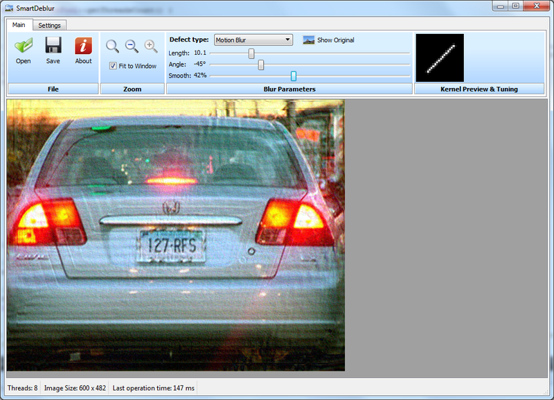
The results show that SmartDeblur produces comparable quality to both commercial tools. The core deconvolution algorithms appear to be similar across all three tools — after all, Wiener filtering is well-established mathematics. The commercial tools likely add post-processing steps such as noise reduction and edge enhancement, which SmartDeblur doesn't yet implement.

Conclusion

The results have exceeded my expectations — even a relatively simple implementation of the Wiener filter produces very usable results for defocus correction. The main challenges lie not in the deconvolution itself, but in correctly estimating the PSF and dealing with edge effects.

The source code is available on GitHub. I should warn that the code quality leaves much to be desired — there are memory leaks and various architectural issues that need refactoring. But it works, and it demonstrates the principles effectively.

I would be grateful for any feedback, bug reports, and suggestions. If there is interest, I plan to write a follow-up article about blind deconvolution — restoring images when the PSF is unknown.