The Integral That Took a Century to Solve

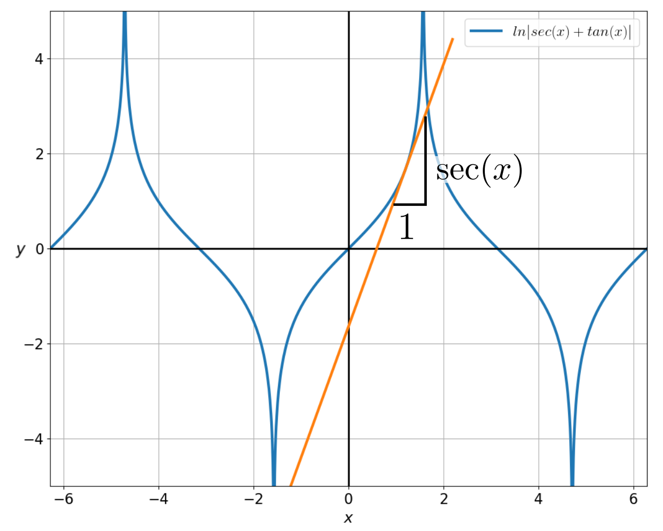
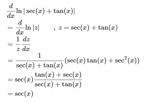
When students encounter the integral ∫sec(x)dx = ln|sec(x) + tan(x)| + c in a first-year calculus course, it seems like a routine formula. Few suspect that establishing this result formally took almost a century—and that the search began not in a mathematician's study, but on a navigator's chart table.

A Quick Trigonometry Refresher

Most trigonometric integrals are straightforward:

• ∫sin(x) dx = −cos(x) + c
• ∫cos(x) dx = sin(x) + c
• ∫tan(x) dx = −ln|cos(x)| + c

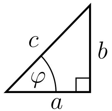
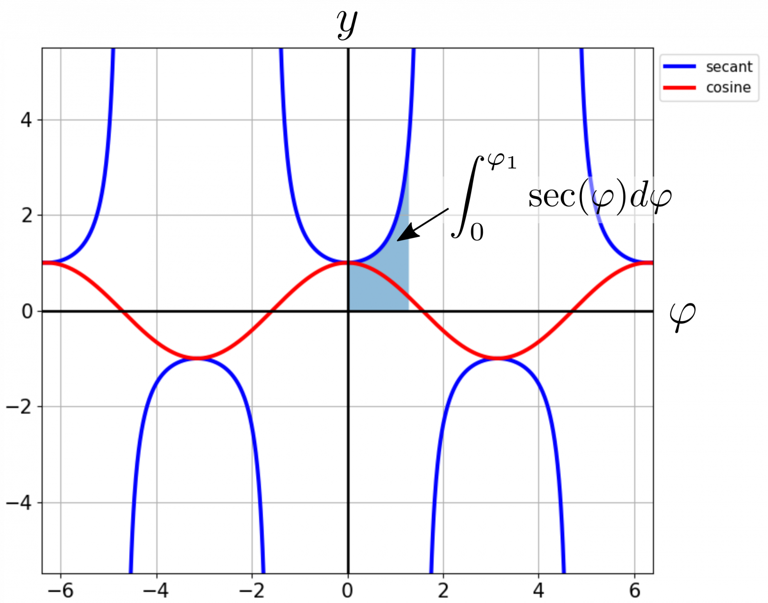
The secant function is defined as sec(φ) = 1/cos(φ), i.e., the ratio of hypotenuse to adjacent side in a right triangle. Geometrically, ∫sec(x) dx represents the area under the secant curve. Simple enough to state—yet devilishly hard to prove.

The Cartography Problem

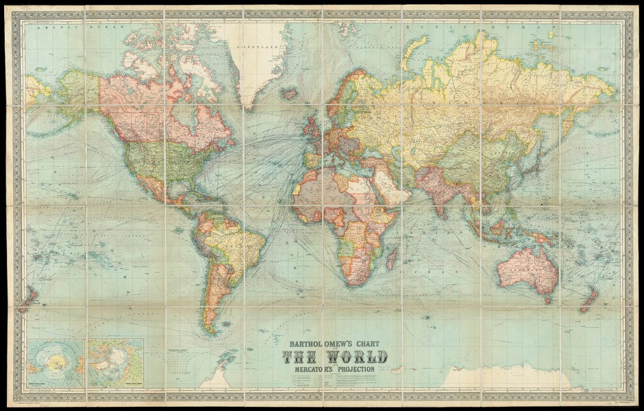
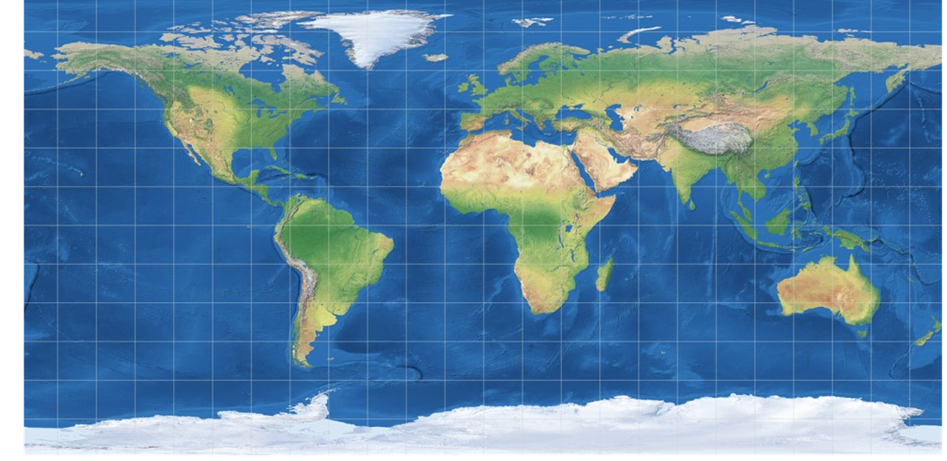
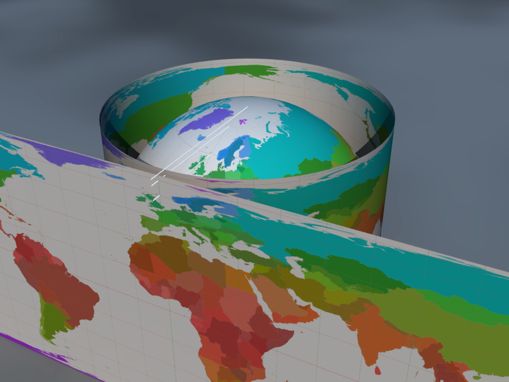
In 1569 Gerard Mercator published his famous world map. His goal was practical: sailors needed a chart where a rhumb line—a path of constant compass bearing—appears as a straight line. That property is invaluable for navigation, but achieving it requires a mathematically precise vertical stretching of the globe onto a flat surface.

Two simpler projections illustrate the difficulty:

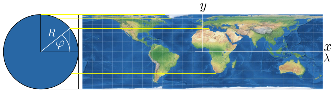
• Equirectangular: y = Rφ, x = Rλ. Simple, but heavily distorts areas away from the equator.
• Lambert's equal-area cylindrical: y = R sin(φ), x = Rλ. Preserves area but distorts shapes near the poles.

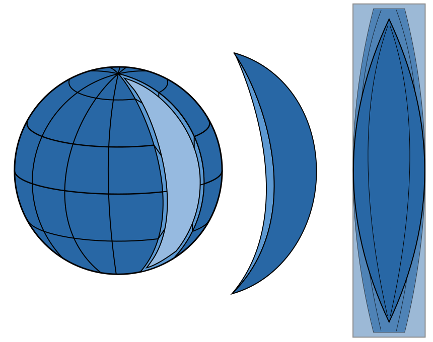
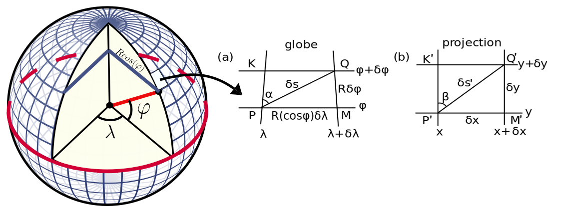
Mercator needed a projection that preserved angles (a conformal projection). To keep angles correct, the horizontal stretching factor at latitude φ is sec(φ). To compensate and maintain conformality, the vertical scale must also be stretched by the same factor, giving an infinitesimal vertical increment:

δy = R · sec(φ) · δφ

The total y-coordinate at latitude φ is therefore:

y = R · ∫₀^φ sec(t) dt

Since calculus did not yet exist, Mercator could only approximate this by summing many thin strips:

y_n ≈ Σ R · sec(k · δφ) · δφ

He computed these sums numerically and drew his map. The result worked, but the underlying formula remained a mystery.

Edward Wright and the First Tables (1599)

English mathematician Edward Wright independently derived the Mercator projection in 1599 and published precise numerical tables of the accumulated secant sums. His tables became the standard reference for navigators but still gave no closed-form answer.

Napier's Logarithms (1614)

John Napier published his tables of logarithms in 1614, giving mathematicians a powerful new computational tool. Within decades, logarithmic-trigonometric tables (log-tangent tables) were widely available.

Bond's Conjecture (1645)

Around 1645, mathematics teacher Henry Bond compared Wright's Mercator tables with the new log-tangent tables. He noticed that every entry in Wright's column matched a corresponding entry in the log-tangent column with a constant offset. Bond proposed the conjecture:

∫₀^φ sec(t) dt = ln| tan(φ/2 + 45°) |

This is believed to be the only important integral in history discovered primarily through numerical pattern observation rather than analytical reasoning. Bond could not prove it—he simply saw it in the numbers.

Gregory's Proof (1668)

Nearly a quarter-century later, in 1668, Scottish mathematician James Gregory provided the first rigorous proof of Bond's conjecture. Gregory's approach, while correct, was described by contemporaries as "tedious and exhausting." Nevertheless, a century-old problem had at last been closed.

Barrow's Elegant Proof (1670)

Just two years later Isaac Barrow—Newton's teacher—found a far more elegant proof using partial fractions. The key manipulation is:

sec(φ) = 1/cos(φ)
       = cos(φ) / cos²(φ)
       = cos(φ) / (1 − sin²(φ))
       = cos(φ) / [(1 − sin(φ))(1 + sin(φ))]

Applying partial fractions:

sec(φ) = ½ · cos(φ)/(1 − sin(φ))  +  ½ · cos(φ)/(1 + sin(φ))

Both terms integrate immediately:

∫ sec(φ) dφ = ½ ln|1 + sin(φ)| − ½ ln|1 − sin(φ)| + c
            = ½ ln|(1 + sin(φ))/(1 − sin(φ))| + c

With trigonometric identities one can verify all three forms are equivalent:

• ln|sec(φ) + tan(φ)| + c
• ln|tan(φ/2 + 45°)| + c
• ½ ln|(1 + sin(φ))/(1 − sin(φ))| + c

Modern Legacy

The Mercator projection remains the backbone of online mapping today. Google Maps, Apple Maps, and OpenStreetMap all use the Web Mercator variant because it preserves local angles, which is essential for street-level navigation and turn-by-turn routing.

The projection's famous flaw—Greenland appearing larger than Africa when the opposite is true—has prompted ongoing debate about whether widely-used map projections carry a subtle colonial bias by over-representing northern continents.

Alternative projections address this in different ways:

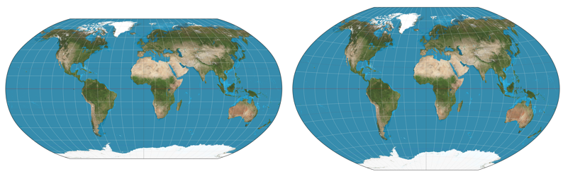
• Winkel Tripel: An elegant mathematical compromise between shape preservation and scale accuracy. Used by National Geographic.
• Robinson: Designed artistically rather than derived analytically—Robinson drew the graticule by hand at 5° intervals to produce a pleasing appearance.

What the History Teaches Us

Mathematics rarely develops as neatly as textbooks suggest. Students encounter the finished formula ∫sec(x) dx = ln|sec(x) + tan(x)| + c and assume it was always known. In reality, its story spans a century, crosses multiple disciplines, and involves a crucial leap made not by deduction but by staring at columns of numbers until a pattern emerged.

The secant integral is a perfect reminder that practical engineering problems—in this case, the desperately practical problem of not getting lost at sea—have driven some of the deepest theoretical advances in mathematics.